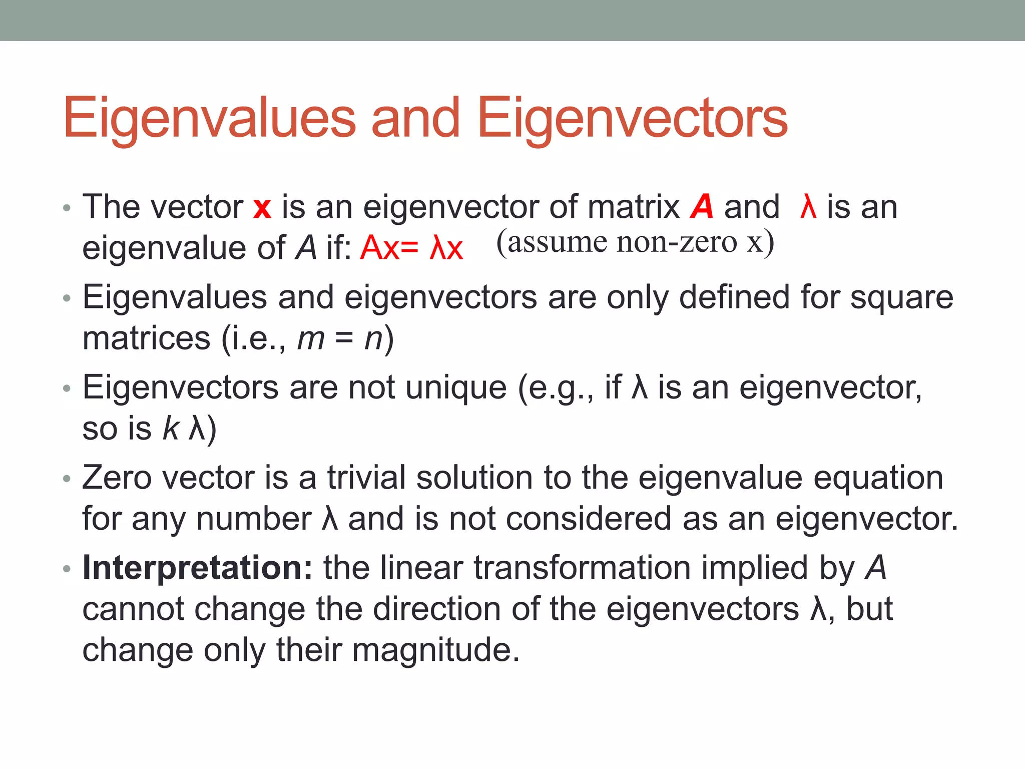
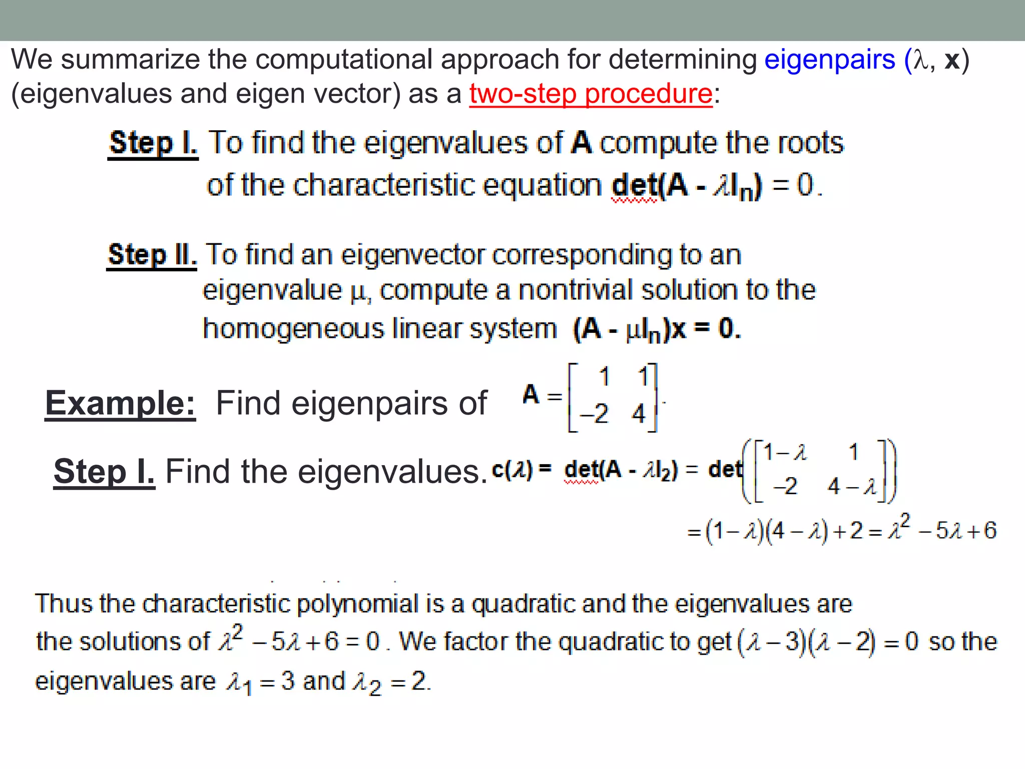
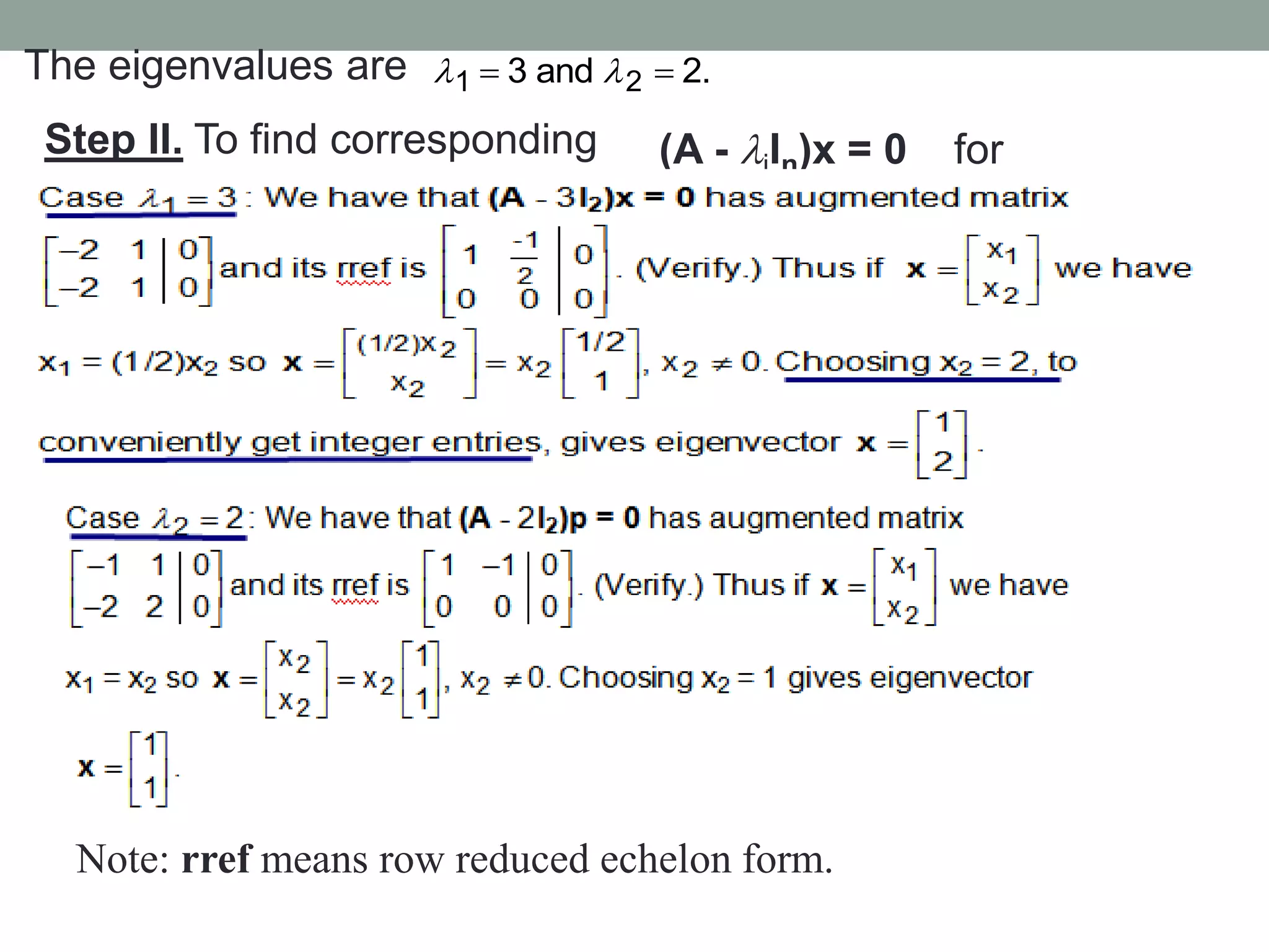
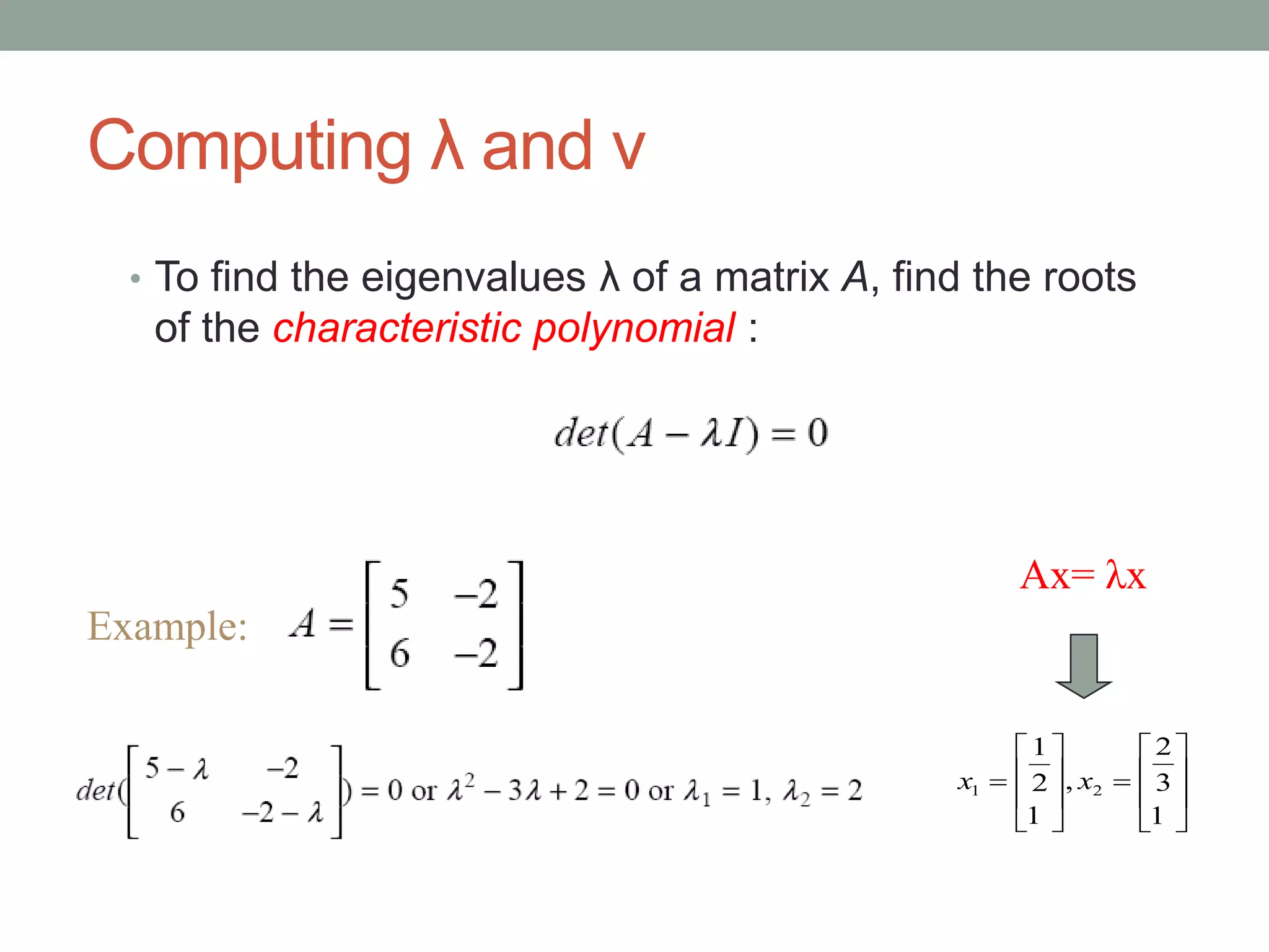
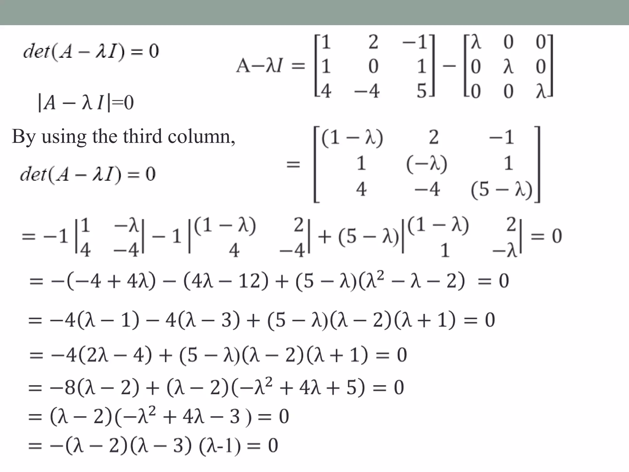
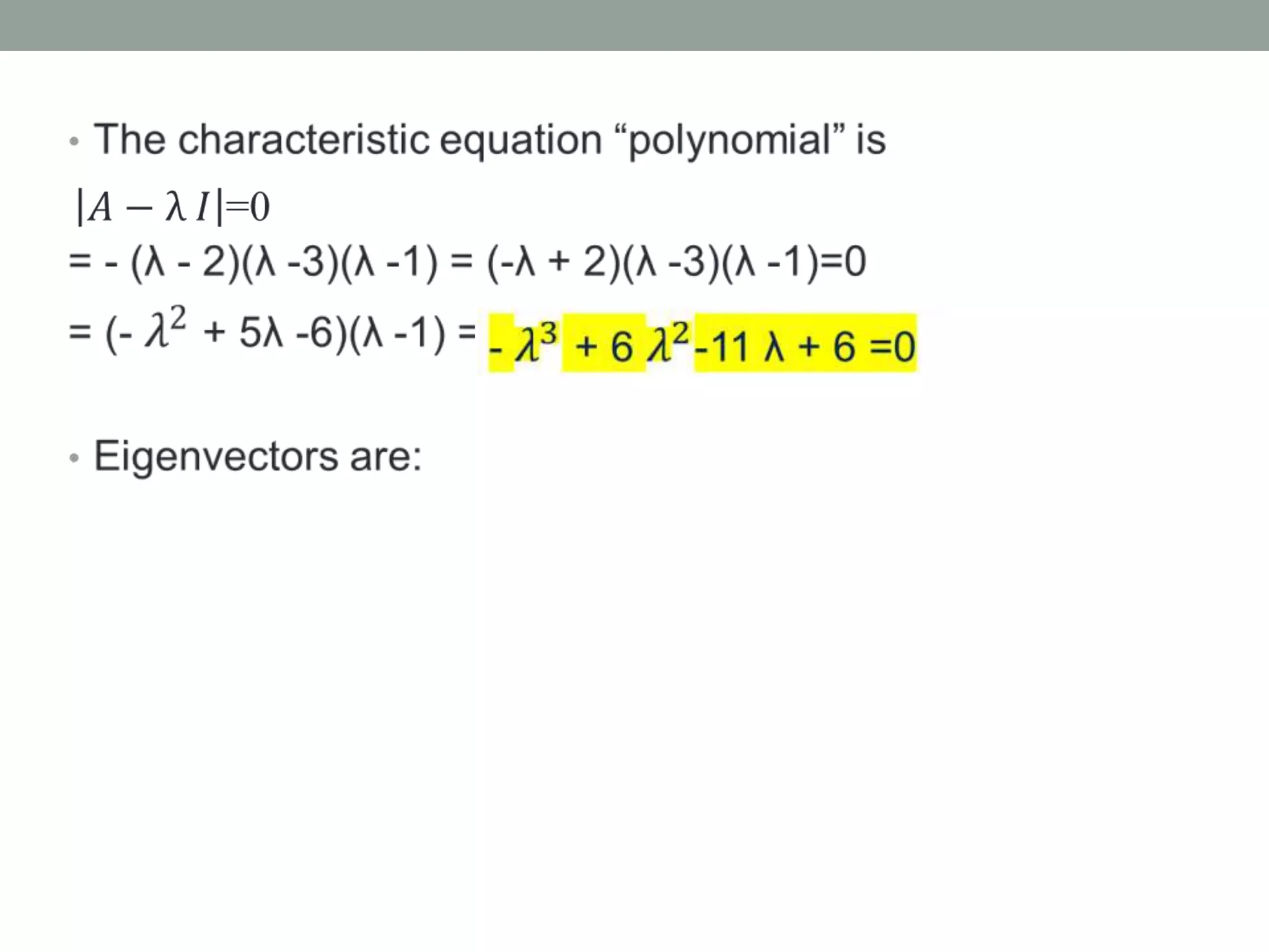
The document discusses the concepts of eigenvalues and eigenvectors, defining an eigenvector as a vector that, when multiplied by a matrix, results in a scalar multiple of itself, alongside the eigenvalue. It outlines a two-step computational approach to determine these components, starting with finding eigenvalues through the characteristic polynomial, followed by solving for eigenvectors. The document emphasizes that eigenvectors are not unique and clarifies that the zero vector is not considered an eigenvector.

1. Eigenvalues and Eigenvectors

2. Eigenvalues and Eigenvectors
• The vector x is an eigenvector of matrix A and λ is an
eigenvalue of A if: Ax= λx
• Eigenvalues and eigenvectors are only defined for square
matrices (i.e., m = n)
• Eigenvectors are not unique (e.g., if λ is an eigenvector,
so is k λ)
• Zero vector is a trivial solution to the eigenvalue equation
for any number λ and is not considered as an eigenvector.
• Interpretation: the linear transformation implied by A
cannot change the direction of the eigenvectors λ, but
change only their magnitude.
(assume non-zero x)

3. We summarize the computational approach for determining eigenpairs (, x)
(eigenvalues and eigen vector) as a two-step procedure:
Example: Find eigenpairs of
Step I. Find the eigenvalues.

4. The eigenvalues are  
1 2
3 and 2.
 
Step II. To find corresponding
eigenvectors we solve
(A - iIn)x = 0 for
i = 1,2
Note: rref means row reduced echelon form.

5. Computing λ and v
• To find the eigenvalues λ of a matrix A, find the roots
of the characteristic polynomial :
Example:
Ax= λx


















1
3
2
,
1
2
1
2
1 x
x

6. Example: Find eigenvalues and eigen vectors of 






0
1
1
0
A
The characteristic polynomial is

7. Example: Find the eigenvalues and corresponding
eigenvectors of
The characteristic polynomial is
Its factors are
So the eigenvalues are 1, 2, and 3.
Corresponding
eigenvectors are

8. By using the third column,