The document provides an overview of microwave radio planning and link design. It discusses topics such as PCM and E1 overview, digital multiplexing standards PDH and SDH, digital microwave systems, microwave link performance objectives, antennas, propagation, planning, interference management, and frequency allocation. The course contents include topology planning, diversity techniques, link budgeting, performance prediction using path profiles and LOS surveys.

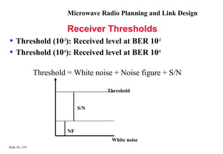
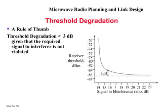
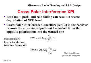
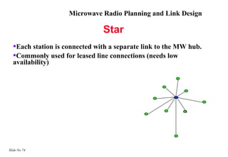
![Microwave Radio Planning and Link Design
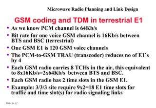
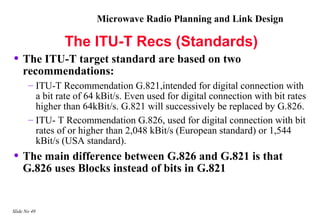
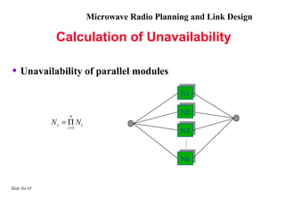
Transmission Capacity Planning-Example
• Example: How Many Motorola micro-cells can be daisy
chained using one E1 at maximum?
• Solution:
– Motorola micro cell has 2 radios (omni-2)
– Each micrcell requires 2x2 time slots for traffic and 1 time slot for
rsl
– So each micro cell requires 5 time slots (64 kb/s time slots)
– Each E1 contains 31 time slots
– [31time slots] divided by [5 time slots/microcell] gives us the the
maximum no of daisy chained microcells
– So 6 microcells can be daisy chained at maximum
Slide No 72](https://image.slidesharecdn.com/52528672-microwave-planning-and-design-130131062113-phpapp01/85/52528672-microwave-planning-and-design-72-320.jpg)

![Microwave Radio Planning and Link Design
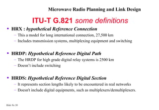
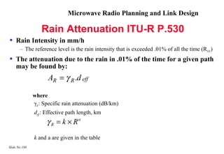
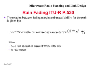
Rain Attenuation
• Rain rate is measured to estimate attenuation because it is
hard to actually count the number of raindrops and
measure their individual sizes so
• Rainfall is measured in millimeters [mm], and rain
intensity in millimeters pr. hour [mm/h].
• Since the radio waves are a time varying electromagnetic
field, the incident field will induce a dipole moment in the
raindrop will therefore act as an antenna and re-radiate
the energy.
• A raindrop is an antenna with low directivity and some
energy will be re-radiated in arbitrary directions giving a
net loss of energy in the direction towards the receiver.
Slide No 146](https://image.slidesharecdn.com/52528672-microwave-planning-and-design-130131062113-phpapp01/85/52528672-microwave-planning-and-design-146-320.jpg)
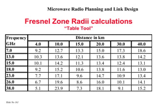
![Microwave Radio Planning and Link Design
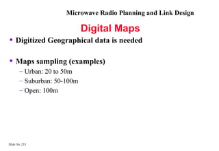
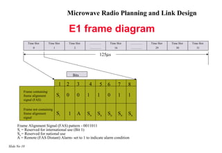
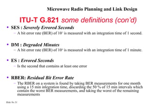
Fresnel Zone Equation
• First Fresnel zone radius
d1 × d 2
F1 = 17.3 × [m]
d× f
• Fresnel zone – Exercise: Calculate the fresnel zone radius at mid
path for the following cases
– 1. f= 15GHz, K=4/3, d=10km
– 2. f = 15GHz, K=4/3, d=20km
• Solution:
= 17.3 ×
5×5
= 7m
– 1. F1 (radius) 15 × 10
10 × 10
= 17.3 × = 10m
– 2. F1 (radius) 15 × 20
Slide No 160](https://image.slidesharecdn.com/52528672-microwave-planning-and-design-130131062113-phpapp01/85/52528672-microwave-planning-and-design-160-320.jpg)
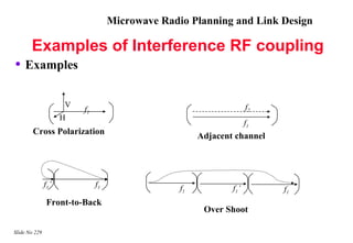
![Microwave Radio Planning and Link Design
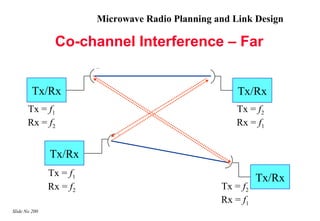
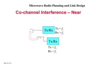
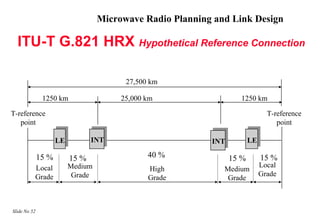
Co-channel arrangement
• In this arrangement every radio channel is utilized twice
for independent traffic on opposite polarization for the
same path
• The following demand must be fulfilled
[10log(1/(1/10^((XPD + XIF)/10) +1/10^((NFD-3)/10)))] > (C/I)
Where,
NFD :Net Filter discriminator
XIF :is XPD improvement factor
Slide No 198](https://image.slidesharecdn.com/52528672-microwave-planning-and-design-130131062113-phpapp01/85/52528672-microwave-planning-and-design-198-320.jpg)