This document provides information about plate heat exchangers (PHEs), including: 1) PHEs consist of a pack of thin corrugated plates that transfer heat between two fluids flowing through narrow channels. 2) PHEs have advantages like flexibility, compact size, efficient heat transfer, and ease of cleaning compared to shell-and-tube heat exchangers. 3) The document discusses mechanical characteristics of PHE components and design considerations for thermal performance and operating limitations.

1. 2,850+
OPEN ACCESS BOOKS
98,000+
INTERNATIONAL
AUTHORS AND EDITORS
91+ MILLION
DOWNLOADS
BOOKS
DELIVERED TO
151 COUNTRIES
AUTHORS AMONG
TOP 1%
MOST CITED SCIENTIST
12.2%
AUTHORS AND EDITORS
FROM TOP 500 UNIVERSITIES
Selection of our books indexed in the
Book Citation Index in Web of Science™
Core Collection (BKCI)
Chapter from the book Heat Transfer Studies and Applications
Downloaded from: http://www.intechopen.com/books/heat-transfer-studies-and-
applications
PUBLISHED BY
World's largest Science,
Technology & Medicine
Open Access book publisher
Interested inpublishing withInTechOpen?
Contact us at book.department@intechopen.com

2. Chapter 7
Modeling and Design of Plate Heat Exchanger
Fábio A.S. Mota, E.P. Carvalho and
Mauro A.S.S. Ravagnani
Additional information is available at the end of the chapter
http://dx.doi.org/10.5772/60885
1. Introduction
Heat exchangers are devices used to transfer energy between two fluids at different temper‐
atures. They improve energy efficiency, because the energy already within the system can be
transferred to another part of the process, instead of just being pumped out and wasted. In the
new era of sustainability, the growing urgency to save energy and reduce overall environ‐
mental impacts has placed greater emphasis on the use of heat exchangers with better thermal
efficiency. In this new scenario, the plate heat exchanger can play an important role.
A plate heat exchanger is a compact type of heat exchanger that uses a series of thin plates to
transfer heat between two fluids. There are four main types of PHE: gasketed, brazed, welded,
and semi-welded. The plate-and-frame or gasketed plate heat exchanger essentially consists
of a pack of thin rectangular plates sealed around the edges by gaskets and held together in a
frame (Figure 1). Plate heat exchangers were first introduced in 1923 for milk pasteurization
applications, but are now used in many applications in the chemical, petroleum, HVAC,
refrigeration, dairy, pharmaceutical, beverage, liquid food and health care sectors. This is due
to the unique advantages of PHEs, such as flexible thermal design (plates can be simply added
or removed to meet different heat duty or processing requirements), ease of cleaning to
maintain strict hygiene conditions, good temperature control (necessary in cryogenic appli‐
cations), and better heat transfer performance.
2. Mechanical characteristics
A PHE consists of a pack of thin rectangular plates with portholes, through which two fluid
streams flow, where heat transfer takes place. Other components are a frame plate (fixed plate),
© 2015 The Author(s). Licensee InTech. This chapter is distributed under the terms of the Creative Commons
Attribution License (http://creativecommons.org/licenses/by/3.0), which permits unrestricted use, distribution,
and reproduction in any medium, provided the original work is properly cited.

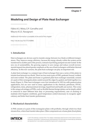
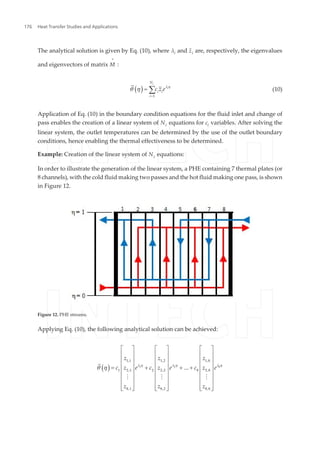
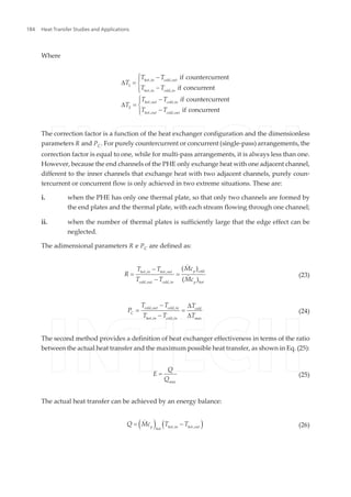
3. a pressure plate (movable plate), upper and lower bars and screws for compressing the pack
of plates (Figure 2). An individual plate heat exchanger can hold up to 700 plates. When the
package of plates is compressed, the holes in the corners of the plates form continuous tunnels
or manifolds through which fluids pass, traversing the plate pack and exiting the equipment.
The spaces between the thin heat exchanger plates form narrow channels that are alternately
traversed by hot and cold fluids, and provide little resistance to heat transfer.
2.1. Thermal plates and gaskets
The most important and most expensive part of a PHE is its thermal plates, which are made
of metal, metal alloy, or even special graphite materials, depending on the application.
Stainless steel, titanium, nickel, aluminum, incoloy, hastelloy, monel, and tantalum are some
examples commonly found in industrial applications. The plates may be flat, but in most
applications have corrugations that exert a strong influence on the thermal-hydraulic per‐
formance of the device. Some of the main types of plates are shown in Figure 3, although the
majority of modern PHEs employ chevron plate types. The channels formed between adjacent
plates impose a swirling motion to the fluids, as can be seen in Figure 4. The chevron angle is
reversed in adjacent sheets, so that when the plates are tightened, the corrugations provide
numerous points of contact that support the equipment. The sealing of the plates is achieved
by gaskets fitted at their ends. The gaskets are typically molded elastomers, selected based on
their fluid compatibility and conditions of temperature and pressure. Multi-pass arrangements
can be implemented, depending on the arrangement of the gaskets between the plates. Butyl
or nitrile rubbers are the materials generally used in the manufacture of the gaskets.
Figure 1. Typical plate heat exchangers [1].
Heat Transfer Studies and Applications166

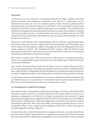
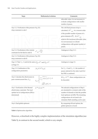
4. Figure 3. Typical cathegories of plate corrugations. (a) washboard, (b) zigzag, (c) chevron or herringbone, (d) protru‐
sions and depressions (e) washboard with secondary corrugations, e (f) oblique washboard [3].
Figure 2. Exploded View of a Plate Heat Exchanger [2].
Modeling and Design of Plate Heat Exchanger
http://dx.doi.org/10.5772/60885
167

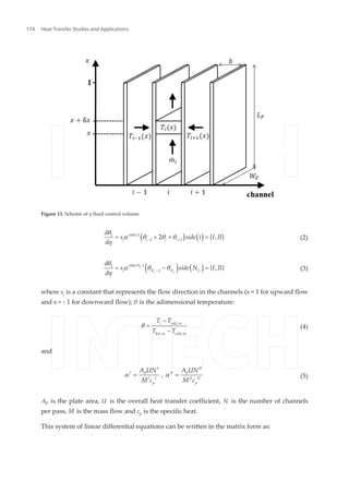
5. Figure 4. Turbulent flow in PHE channels [4].
2.2. Design characteristics
This section presents some of the main advantages and disadvantages of a PHE, compared to
shell-and-tube heat exchangers.
Advantages
Flexibility: Simple disassembly enables the adaptation of PHEs to new process requirements
by simply adding or removing plates, or rearranging the number of passes. Moreover, the
variety of patterns of plate corrugations available, together with the possibility of using
combinations of them in the same PHE, means that various conformations of the unit can be
tested during optimization procedures.
Good temperature control: Due to the narrow channels formed between adjacent plates, only a
small volume of fluid is contained in a PHE. The device therefore responds rapidly to changes
in process conditions, with short lag times, so that the temperatures are readily controllable.
This is important when high temperatures must be avoided. Furthermore, the shape of the
channels reduces the possibility of stagnant zones (dead space) and areas of overheating.
Low manufacturing cost: As the plates are only pressed (or glued) together, rather than welded,
PHE production can be relatively inexpensive. Special materials may be used to manufacture
the plates in order to make them more resistant to corrosion and/or chemical reactions.
Efficient heat transfer: The corrugations of the plates and the small hydraulic diameter enhance
the formation of turbulent flow, so that high rates of heat transfer can be obtained for the fluids.
Consequently, up to 90% of the heat can be recovered, compared to only 50% in the case of
shell-and-tube heat exchangers.
Compactness: The high thermal effectiveness of PHEs means that they have a very small
footprint. For the same area of heat transfer, PHEs can often occupy 80% less floor space
(sometimes 10 times less), compared to shell-and-tube heat exchangers (Figure 5).
Heat Transfer Studies and Applications168

6. Figure 5. Illustration of the typical size difference between a PHE and a shell-and-tube heat exchanger for a given heat
load [5].
Reduced fouling: Reduced fouling results from the combination of high turbulence and a short
fluid residence time. The scale factors for PHEs can be up to ten times lower than for shell-
and-tube heat exchangers.
Ease of inspection and cleaning: Since the PHE components can be separated, it is possible to
clean and inspect all the parts that are exposed to fluids. This feature is essential in the food
processing and pharmaceutical industries.
Easy leak detection: The gaskets have vents (Figure 6) that prevent fluids from mixing in the case
of a failure, which also facilitate locating leaks.
Figure 6. Vents in gaskets to detect possible leaks [4].
Modeling and Design of Plate Heat Exchanger
http://dx.doi.org/10.5772/60885
169

7. Drawbacks
Temperature and pressure limitations: An important limitation of PHEs is related to the plate
gaskets. Pressures and temperatures exceeding 25 atm and 160 °C, respectively, are not
tolerated because they can cause the standard gaskets to leak. However, gaskets made of
special materials can withstand temperatures up to 400 °C, and it is possible to weld or braze
the plates to each other in order to operate under more severe conditions. This would have the
additional advantages of increasing the operational limits, as well as the possibility of working
with corrosive fluids, because it would eliminate the need for gaskets. However, the PHE
would lose its major advantages of flexibility and ease of cleaning, and the equipment would
become more expensive.
High pressure drop: Because of the corrugated plates and the small flow space between them,
the pressure drop due to friction is high, which increases pumping costs. The pressure drop
can be reduced by increasing the number of passages per pass and splitting the flow into a
greater number of channels. This diminishes the flow velocity within the channel, hence
reducing the friction factor. However, the convective heat transfer coefficient is also reduced,
decreasing the effectiveness of the heat exchanger.
Phase change: In special cases, PHEs can be used in condensation or evaporation operations,
but are not recommended for gases and vapors due to the limited space within the channels
and pressure limitations.
Types of fluids: The processing of fluids that are highly viscous or contain fibrous material is
not recommended because of the high associated pressure drop and flow distribution prob‐
lems within the PHE. Compatibility between the fluid and the gasket material should also be
considered. Highly flammable or toxic fluids must be avoided due to the possibility of leakage.
Leakage: Friction between the metal plates can cause wear and the formation of small holes that
are difficult to locate. As a precaution, it is advisable to pressurize the process fluid so that
there is less risk of contamination in the event of leakage from a plate.
2.3. Arrangement of a plate heat exchanger
The simplest types of arrangements of plate heat exchangers are those in which both fluids
make just one pass, so there is no change in direction of the streams. These are known as 1-1
single-pass arrangements, and there are two types: countercurrent and concurrent. A great
advantage of the single-pass arrangement is that the fluid inlets and outlets can be installed in
the fixed plate, making it easy to open the equipment for maintenance and cleaning, without
disturbing the pipework. This is the most widely used single-pass design, known as the U-
arrangement. There is also a single-pass Z-arrangement, where there is input and output of
fluids through both end plates (Figure 7).
Countercurrent flow, where the streams flow in opposite directions, is usually preferred due
the achievement of higher thermal efficiency, compared to concurrent flow, where the streams
flow in the same direction. Multi-pass arrangements can also be employed to enhance the heat
Heat Transfer Studies and Applications170

8. transfer or flow velocity of the streams, and are usually required when there is a substantial
difference between the flow rates of the streams (Figure 8).
Figure 8. Multi-pass PHE.
There are five parameters that can be used to characterize the PHE configuration [6]: NC, P I
,
P II
, ϕ, Yh and Yf .
Number of channels (NC): The space between two adjacent plates is a channel. The end plates
are not considered, so the number of channels of a PHE is the number of plates minus one. The
odd-numbered channels belong to side I, and the even-numbered ones belong to side II (Figure
9). The number of channels in each side are NC
I
and NC
II
.
Number of passes (P): This is the number of changes of direction of a determined stream inside
the plate pack, plus one. P I
and P II
are the number of passes in each side.
Hot fluid location (Yh ): It is a binary parameter that assigns the fluids to the PHE sides. If Yh
= 1 the hot fluid occupies side I while if Yh = 0 the hot fluid occupies side II.
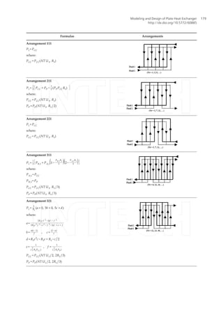
Feed connection (ϕ): Feed side I is arbitrarily set at η = 0 as presented in Figure 9. The parameter
ϕ represents the relative position of side II. Figure 9 illustrates all possibilities of connection.
The parameter η is defined as η = x / L P.
Figure 7. Arrangements of a simple-pass PHE. (a) U-arrangement and (b) Z-arrangement.
Modeling and Design of Plate Heat Exchanger
http://dx.doi.org/10.5772/60885
171

9. Figure 9. Feed connection of a PHE.
The plates of a PHE can provide vertical or diagonal flow, depending on the arrangement of
the gaskets. For vertical flow, the inlet and outlet of a given stream are located on the same
side of the heat exchanger, whereas for diagonal flow they are on opposite sides. Assembly of
the plate pack involves alternating between the “A” and “B” plates for the respective flows.
Mounting of the plate pack in vertical flow mode only requires an appropriate gasket config‐
uration, because the A and B arrangements are equivalent (they are rotated by 180°, as shown
in Figure 10a). This is not possible in the case of diagonal flow, which requires both types of
mounting plate (Figure 10b). To identify each type of flow, Gut (2003) considered the binary
parameter Yf (Yf = 1 for diagonal flow and Yf = 0 for vertical flow). Poor flow distribution is
more likely to occur in the array of vertical flow [7].
Figure 9. Feed connection of a PHE.
The plates of a PHE can provide vertical or diagonal flow, depending on the arrangement of the gaskets. For vertical
flow, the inlet and outlet of a given stream are located on the same side of the heat exchanger, whereas for diagonal flow
they are on opposite sides. Assembly of the plate pack involves alternating between the “A” and “B” plates for the
respective flows. Mounting of the plate pack in vertical flow mode only requires an appropriate gasket configuration,
because the A and B arrangements are equivalent (they are rotated by 180°, as shown in Figure 10a). This is not
possible in the case of diagonal flow, which requires both types of mounting plate (Figure 10b). To identify each type of
flow, Gut (2003) considered the binary parameter ( = 1 for diagonal flow and = 0 for vertical flow). Poor flow
distribution is more likely to occur in the array of vertical flow [7].
(a)
(b)
Figure 10a. Vertical flow plate [9]. Figure 10b. Diagonal flow plate [9].
3. MATHEMATICAL MODELING
Due to the large number of plate types and pass arrangements, there are many possible configurations of a particular
PHE design. As a result, a number of mathematical modeling approaches have been proposed for the calculation of
performance. Two different modeling approaches are described below.
Figure 10. (a). Vertical flow plate [9]. (b). Diagonal flow plate [9].
Heat Transfer Studies and Applications172

10. 3. Mathematical modeling
Due to the large number of plate types and pass arrangements, there are many possible
configurations of a particular PHE design. As a result, a number of mathematical modeling
approaches have been proposed for the calculation of performance. Two different modeling
approaches are described below.
3.1. Model 1
A mathematical model was developed to simulate the general configuration of a PHE oper‐
ating under steady state conditions, characterized using six different parameters [6]. In this
model, the parameters considered are the number of channels, the number of passes for each
side, the fluid locations, the feed connection locations, and the type of channel flow. The
following assumptions are made:
• The PHE operates at steady state;
• The main flow is divided equally among the channels that make up each pass;
• The velocity profile in the channels is flat (plug flow);
• Perfect mixture in the end of each pass;
• There are no heat losses to the environment;
• There are no phase change;
• There is no heat transfer in the direction of flow, either in the fluids or in the plates, so heat
transfer only occurs in the direction perpendicular to the flow;
• The physical properties of the fluids remain constant throughout the process.
The last assumption listed above implies an overall heat transfer coefficient U constant
throughout the process, which is quite reasonable for compact heat exchangers operating
without phase change [10]. In the absence of this consideration, the energy balance in the
channels would result in a nonlinear system of ordinary first order differential equations,
which would make the simulation much more complex. It has also been found that the results
obtained assuming a constant overall heat transfer coefficient are very close to those found
without such a restriction [6]. Thus, this assumption is not a limiting factor for the evaluation
of a PHE.
Applying the energy conservation law to a given volume of control of a generic channel i with
dimensions WP, δx and b (Figure 11) and neglecting variations of kinetic and potential energy,
the enthalpy change of the fluid passing through the volume is equal to the net heat exchanged
by the two adjacent channels. This can be described by a system of differential equations:
( )Id
s
d
1
1 2 1
q
a q q
h
= - (1)
Modeling and Design of Plate Heat Exchanger
http://dx.doi.org/10.5772/60885
173

11. ( ) ( )side i
i i i i
d
s side i I II
d
( )1
1 1
2 { , }
q
a q q q
h - +
= + + = (2)
( ) ( )C
c c
side N
i N N C
d
s side N I II
d
( )1
1
{ , }
q
a q q
h -
= - = (3)
where si is a constant that represents the flow direction in the channels (s = 1 for upward flow
and s = - 1 for downward flow); θ is the adimensional temperature:
i cold in
hot in cold in
T T
T T
,
, ,
q
-
=
-
(4)
and
I II
I IIP P
I I II II
p p
A UN A UN
M c M c
,a a= =
& & (5)
AP is the plate area, U is the overall heat transfer coefficient, N is the number of channels
per pass, M˙ is the mass flow and cp is the specific heat.
This system of linear differential equations can be written in the matrix form as:
Figure 11. Scheme of a fluid control volume
Heat Transfer Studies and Applications174

12. d
M
d
.
q
q
h
=
= (6)
where
C C C
C C
N N N
N N
d d
d d d
d d d
M
d d d
d d
1 1
2 2 2
3 3 3
1 1 1
0 0 0
2 0 0
0 2
0
0 0 2
0 0 0
=
- - -
é ù- +
ê ú
+ - +ê ú
ê ú+ - +
ê ú=
ê ú
ê ú+ - +
ê ú
ê ú+ -
ë û
L
L
M
M
L
L
I
i
i CII
i
s i
d i N
s i i
[ if is odd
1,...,
f is even
a
a
ìï
= =í
ïî
The boundary conditions, which are dependent on the PHE configuration, can be divided into
three different categories:
1. Fluid inlet temperature: In the channels of the first pass, the fluid inlet temperature is the
fluid feed temperature.
( )i fluid in
i,
first passq h q= ò (7)
2. Change of pass temperature: The temperature at the beginning of the channels of a particular
pass is equal to the arithmetic average of the temperatures in the channels of the previous
pass.
( ) ( )
N
i j
j previous
pass
i
N
1
new passq h q h= åò
ò
(8)
3. Fluid outlet temperature: The outlet temperature of the fluid is the arithmetic average of the
outlet temperatures of the channels of the last pass.
( ) ( )
N
fluid out j
j last
pass
N,
1
q h q h= åò
(9)
Modeling and Design of Plate Heat Exchanger
http://dx.doi.org/10.5772/60885
175

13. The analytical solution is given by Eq. (10), where λi and z¯i are, respectively, the eigenvalues
and eigenvectors of matrix M
=
:
( )
c
i
N
i i
i
c z e
1
l h
q h
=
= å (10)
Application of Eq. (10) in the boundary condition equations for the fluid inlet and change of
pass enables the creation of a linear system of Nc equations for ci variables. After solving the
linear system, the outlet temperatures can be determined by the use of the outlet boundary
conditions, hence enabling the thermal effectiveness to be determined.
Example: Creation of the linear system of Nc equations:
In order to illustrate the generation of the linear system, a PHE containing 7 thermal plates (or
8 channels), with the cold fluid making two passes and the hot fluid making one pass, is shown
in Figure 12.
Figure 12. PHE streams.
Applying Eq. (10), the following analytical solution can be achieved:
( )
z z z
c z e c z e c z e
z z z
81 2
1,1 1,2 1,8
1 2,1 2 2,2 8 2,8
8,1 8,2 8,8
... l hl h l h
q h
é ù é ù é ù
ê ú ê ú ê ú
ê ú ê ú ê ú
ê ú ê ú ê ú= + + +
ê ú ê ú ê ú
ê ú ê ú ê ú
ê ú ê ú ê ú
ê ú ê ú ê úë û ë û ë û
M M M
Heat Transfer Studies and Applications176

14. Using the boundary condition equations (7) and (8) for all the channels of the PHE under
investigation, the equations presented in Table 1 are generated.
Cold fluid Hot fluid
θ1
(η =0)= θ5
(η =0) + θ7
(η =0) /2 θ2
(η =1)=θhot,in =1
θ3
(η =0)= θ5
(η =0) + θ7
(η =0) /2 θ4
(η =1)=θhot,in =1
θ5
(η =1)=θcold,in =0 θ6
(η =1)=θhot,in =1
θ7
(η =1)=θcold,in =0 θ8
(η =1)=θhot,in =1
Table 1. Boundary condition equations.
These equations can be written in the following way:
( ) ( ) ( )
( )
( ) ( ) ( )
( )
( )
( )
( )
( )
1 5 7
2
3 5 7
4
5
6
7
8
0 0 0 / 2 0
1 1
0 0 0 / 2 0
1 1
1 0
1 1
1 0
1 1
q h q h q h
q h
q h q h q h
q h
q h
q h
q h
q h
é ù= - = + = =ë û
= =
é ù= - = + = =ë û
= =
= =
= =
= =
= =
To achieve the matrix form is Eq. (10) is applied to the linear system:
A C B.
=
= (11)
where
A
=
= eigenvalues and eigenvectors matrix
C¯ =ci ' s coefficients vector
B¯ = binary vector
where
i i hot in
i i cold in
N
i i i j
j previous pass
B B i
B B i
B B
N
,
,
0 if first pass
1 if first pass
1
0 if ( ) ( )
q
q
q h q h
Î
= = Î
= = Î
= = - å
Modeling and Design of Plate Heat Exchanger
http://dx.doi.org/10.5772/60885
177

15. 3.2. Model 2
The assumption is made that any multi-pass PHE with a sufficiently large number of plates
(so that end effects and inter-pass plates can be neglected) can be reduced to an arrangement
consisting of assemblies of single-pass PHEs [11]. This enables the development of closed-form
equations for effectiveness, as a function of the ratio between the heat capacities of the fluids
and the number of transfer units, for the arrangements 1-1, 2-1, 2-2, 3-1, 3-2, 3-3, 4-1, 4-2, 4-3,
and 4-4 (Table 2). In other words, most multi-pass plate heat exchangers can be represented
by simple combinations of pure countercurrent and concurrent exchangers, so that a multi-
pass PHE is therefore equivalent to combinations of smaller single-pass exchangers (Figure 13).
Figure 13. Equivalent configurations.
The assumptions considered are the same as in the first mathematical model. The derived
formulas are only valid for PHEs with numbers of thermal plates sufficiently large that the
end effects can be neglected. This condition can be satisfied, depending on the required degree
of accuracy. For example, a minimum of 19 plates is recommended for an inaccuracy of up to
2.5% [12]. Elsewhere, a minimum of 40 thermal plates was used [11, 13]. In the formulas, PCC
and PP are the thermal effectiveness for the countercurrent and concurrent flows, respectively,
given by:
( )
( )
( )
NTU R
NTU R
CC
e
se R
R e
P NTU R
NTU
se R
NTU
1 1
1 1
1
11
1
1 1
1
1
1
1
1
1
,
1
1
- -
- -
ì -
¹ï
-ï
ï
ï
= í
ï
ï
ï =
ï +î
(12)
( )
( )NTU R
P
e
P NTU R
R
1 11
1 1
1
1
,
1
- +
-
=
+
(13)
Heat Transfer Studies and Applications178

16. Formulas Arrangements
Arrangement 111
P1 = PCC
where:
PCC = PCC(NT U1, R1)
Arrangement 211
P1 =
1
2 PCC + PP −
1
2 (PP PCC R1)
where:
PCC = PCC(NT U1, R1)
PP = PP(NT U1, R1 /2)
Arrangement 221
P1 = PCC
where:
PCC = PCC(NT U1, R1)
Arrangement 311
P1 =
1
3 PB,1 + PA,1
(1−
PB,1R1
3
)(2−
PA,1R1
3
)
where:
PA,1 = PCC
PB,1 = PP
PCC = PCC(NT U1, R1 /3)
PP = PP(NT U1, R1 /3)
Arrangement 321
P1 =
1
R1
(a + 0, 5b + 0, 5c + d)
where:
a=
2R1e f 2
− 2ef − f 2
2R1e 2
f 2
− e 2
− f 2
− 2ef + e + f
b=
a(e − 1)
f , c =
(1 − a)
e
d = R1e 2
c − R1e + R1 −c /2
e =
1
(
2
3 R1PCC)
, f =
1
(
2
3 R1PP)
PCC = PCC(NT U1 /2, 2R1 /3)
PP = PP(NT U1 /2, 2R1 /3)
Modeling and Design of Plate Heat Exchanger
http://dx.doi.org/10.5772/60885
179

17. Formulas Arrangements
Arrangement 331
P1 = PCC
where:
PCC = PCC(NT U1, R1)
Arrangement 411
P1 = PI −
PI
2R1
4
where:
PI =
1
2
(PCC + PP −
R1PCC PP
4
)
PCC = PCC(NT U1, R1 /4)
PP = PP(NT U1, R1 /4)
Arrangement 421
P1 = PI −
PI (1 − PI )(1 − PI R1)
1 − PI
2R1
where:
PI =
1
2
(PCC + PP −
PCC PP R1
2
)
PCC = PCC(NT U1 /2, R1 /2)
PP = PP(NT U1 /2, R1 /2)
Arrangement 431
P1 = A +
BD(1 − G) + BQE
(1 − G)(1 − E) − QS
where:
A=
1
4 (3PCC + PP −rPCC PP)
B =1− A
D =
1
6 (1−rPCC)(3PCC + 3PP −2rPCC PP −rPP
2)
E =
1
12 (1−rPCC)(3−2rPCC −rPP)(PCC + 3PP −rPCC PP −2rPP
2)
G =
r
6 (PCC
2 + 3PP
2) + PCC PP(3−rPCC −2rPP)
H =
r
6 3PCC
2 + PP
2 + PCC PP(3−2rPCC −rPP)
Q =1−
(PCC + PP)
2 +
r PCC PP
3
S =
Er PCC
1 − r PCC
+
r PP
12 (PCC + 3PP −rPP(PCC + 2PP))
r =
3R1
4
PCC = PCC(NT U1 /3, r)
PP = PP(NT U1 /3, r)
Heat Transfer Studies and Applications180

18. Formulas Arrangements
Arrangement 441
P1 = PCC
where:
PCC = PCC(NT U1, R1)
Table 2. Closed formulas for multi-pass arrangement [11]
4. Design of a plate heat exchanger
4.1. Basic equations for the design of a plate heat exchanger
The methodology employed for the design of a PHE is the same as for the design of a tubular
heat exchanger. The equations given in the present chapter are appropriate for the chevron
type plates that are used in most industrial applications.
4.1.1. Parameters of a chevron plate
The main dimensions of a chevron plate are shown in Figure 14. The corrugation angle, β,
usually varies between extremes of 25° and 65° and is largely responsible for the pressure drop
and heat transfer in the channels.
Figure 14. Parameters of a chevron plate.
Modeling and Design of Plate Heat Exchanger
http://dx.doi.org/10.5772/60885
181

19. The corrugations must be taken into account in calculating the total heat transfer area of a plate
(effective heat transfer area):
P P P
A W LΦ. .= (14)
where
AP = plate effective heat transfer area
Φ = plate area enlargement factor (range between 1.15 and 1.25)
WP = plate width
LP = plate length
The enlargement factor of the plate is the ratio between the plate effective heat transfer area,
AP and the designed area (product of length and width WP.L P), and lies between 1.15 and 1.25.
The plate length L P and the plate width WP can be estimated by the orifices distances. L V ,
L H , and the port diameter Dp are given by Eq. (15) and Eq. (16) [5].
P V p
L L D» - (15)
P H p
W L D» + (16)
For the effective heat transfer area, the hydraulic diameter of the channel is given by the
equivalent diameter, De, which is given by:
e
b
D
2
Φ
= (17)
where b is the channel average thickness.
4.1.2. Heat transfer in the plates
The heat transfer area is expressed as the global design equation:
M
Q UA T= D (18)
where U is the overall heat transfer coefficient, A is the total area of heat transfer and ΔTM is
the effective mean temperature difference, which is a function of the inlet and outlet fluid
Heat Transfer Studies and Applications182

20. temperatures, the specific heat, and the configuration of the exchanger. The total area of heat
transfer can be given by:
P P
A N A= (19)
where NP is the number of plates. The end plates, which do not exchange heat, are not taken
into account in determining the area. The inner plates are usually called thermal plates in order
to distinguish them from the adiabatic end plates. The overall heat transfer coefficient can be
determined by:
P
f cold f hot
hot P cold
U
t
R R
h k h , ,
1
1 1
=
+ + + +
(20)
where
hhot = convective heat transfer coefficient of the hot fluid
hcold = convective heat transfer coefficient of the cold fluid
tP = plate thickness
kP = plate thermal conductivity
R f ,hot = fouling factor of the hot fluid
R f ,cold = fouling factor of the cold fluid
The convective heat transfer coefficient, h , depends on the fluid properties, fluid velocity, and
plate geometry.
4.1.3. Design methods
There are two main approaches used in the design of PHEs, namely the log-mean temperature
difference and the thermal effectiveness methods. For the first method, the rate of heat transfer
is given by:
lm
Q UA F T( )= D (21)
where ΔTlm is the log-mean temperature difference, given by Eq. (22) and F is the log-mean
temperature difference correction factor.
( )lm
T T
T
ln T T
1 2
1 2
/
D - D
D =
D D
(22)
Modeling and Design of Plate Heat Exchanger
http://dx.doi.org/10.5772/60885
183

21. Where
hot in cold out
hot in cold in
hot out cold in
hot out cold out
T T
T
T T i
T T i
T
T T
, ,
1
, ,
, ,
2
, ,
if countercurrent
f concurrent
f countercurrent
if concurrent
ì -ï
D = í
-ïî
ì -ï
D = í
-ïî
The correction factor is a function of the heat exchanger configuration and the dimensionless
parameters R and PC. For purely countercurrent or concurrent (single-pass) arrangements, the
correction factor is equal to one, while for multi-pass arrangements, it is always less than one.
However, because the end channels of the PHE only exchange heat with one adjacent channel,
different to the inner channels that exchange heat with two adjacent channels, purely coun‐
tercurrent or concurrent flow is only achieved in two extreme situations. These are:
i. when the PHE has only one thermal plate, so that only two channels are formed by
the end plates and the thermal plate, with each stream flowing through one channel;
ii. when the number of thermal plates is sufficiently large that the edge effect can be
neglected.
The adimensional parameters R e PC are defined as:
p coldhot in hot out
cold out cold in p hot
McT T
R
T T Mc
, ,
, ,
( )
( )
-
= =
-
&
& (23)
cold out cold in cold
C
hot in cold in max
T T T
P
T T T
, ,
, ,
- D
= =
- D
(24)
The second method provides a definition of heat exchanger effectiveness in terms of the ratio
between the actual heat transfer and the maximum possible heat transfer, as shown in Eq. (25):
max
Q
E
Q
= (25)
The actual heat transfer can be achieved by an energy balance:
( ) ( )p hot in hot out
hot
Q Mc T T, ,
= -& (26)
Heat Transfer Studies and Applications184

22. ( ) ( )p cold out cold incold
Q Mc T T, ,
= -& (27)
Thermodynamically, Qmax represents the heat transfer that would be obtained in a pure
countercurrent heat exchanger with infinite area. This can be expressed by:
( )max p max
min
Q Mc T= D& (28)
Using Eqs. (26), (27) and (28), the PHE effectiveness can be calculated as the ratio of tempera‐
tures:
hot
cold
T
R
T
E
T
R
T
max
max
if 1
if 1
ì D
>ï
Dï
= í
Dï <
ïDî
(29)
The effectiveness depends on the PHE configuration, the heat capacity rate ratio (R), and the
number of transfer units (NTU). The NTU is a dimensionless parameter that can be considered
as a factor for the size of the heat exchanger, defined as:
p min
UA
NTU
Mc( )
=
& (30)
4.1.4. Pressure drop in a plate heat exchanger
The pressure drop is an important parameter that needs to be considered in the design and
optimization of a plate heat exchanger. In any process, it should be kept as close as possible to
the design value, with a tolerance range established according to the available pumping power.
In a PHE, the pressure drop is the sum of three contributions:
1. Pressure drop across the channels of the corrugated plates.
2. Pressure drop due to the elevation change (due to gravity).
3. Pressure drop associated with the distribution ducts.
The pressure drop in the manifolds and ports should be kept as low as possible, because it is
a waste of energy, has no influence on the heat transfer process, and can decrease the uni‐
formity of the flow distribution in the channels. It is recommended to keep this loss lower than
10% of the available pressure drop, although in some cases it can exceed 30% [3].
V C P
V
e
fL PG G
P gL
D
2 2
2
1,4
2
r
r r
D = + + (31)
Modeling and Design of Plate Heat Exchanger
http://dx.doi.org/10.5772/60885
185

23. where f is the Fanning fator, given by Eq. (33), P is the number of passes and GP is the fluid
mass velocity in the port, given by the ratio of the mass flow, M˙ , and the flow cross-sectional
area, πDP
2 /4.
P
P
M
G
D 2
4
p
=
&
(32)
p
m
K
f
Re
= (33)
The values for Kp and m are presented in Table 3 as function of the Reynolds number for some
β values.
4.1.5. Experimental heat transfer and friction correlations for the chevron plate PHE
Due to the wide range of plate designs, there are various parameters and correlations available
for calculations of heat transfer and pressure drop. Despite extensive research, there is still no
generalized model. There are only certain specific correlations for features such as flow
patterns, parameters of the plates, and fluid viscosity, with each correlation being limited to
its application range. In this chapter, the correlation described in [14] was used.
n
h
w
Nu C Re Pr
0,17
1/3
( ) ( )
m
m
æ ö
= ç ÷ç ÷
è ø
(34)
where μw is the viscosity evaluated at the wall temperature and the dimensionless parameters
Nusselt number (Nu), Reynolds number (Re) and Prandtl number (Pr) can be defined as:
pe C e
chD G D
Nu Re Pr
k k
, ,
m
m
= = = (35)
In Reynolds number equation, GC is the mass flow per channel and may be defined as the ratio
between the mass velocity per channel m˙ and the cross sectional area of the flow channel
(bWP):
C
P
m
G
bW
=
&
(36)
The constants Ch and n, which depend on the flow characteristics and the chevron angle, are
given in Table 3.
Heat Transfer Studies and Applications186

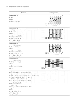
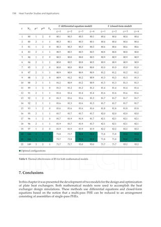
24. 4.2. Optimization
Any industrial process, whether at the project level or at the operational level, has aspects that
can be enhanced. In general, the optimization of an industrial process aims to increase profits
and/or minimize costs. Heat exchangers are designed for different applications, so there can
be multiple optimization criteria, such as minimum initial and operational costs, minimum
volume or area of heat transfer, and minimum weight (important for space applications).
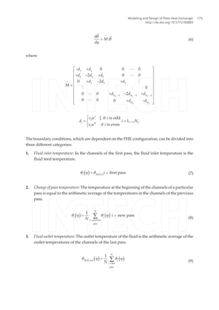
β
Heat transfer Pressure drop
Re Ch n Re K p m
≤ 30°
≤ 10 0.718 0.349 ≤ 10 50.000 1.000
> 10 0.348 0.663 10 - 100 19.400 0.589
> 100 2.990 0.183
45 °
< 10 0.718 0.349 < 15 47.000 1.000
10 - 100 0.400 0.598 15 - 300 18.290 0.652
> 100 0.300 0.663 > 300 1.441 0.206
50 °
< 20 0.630 0.333 < 20 34.000 1.000
20 - 300 0.291 0.591 20 - 300 11.250 0.631
> 300 0.130 0.732 > 300 0.772 0.161
60 °
< 20 0.562 0.326 < 40 24.000 1.000
20 - 200 0.306 0.529 40 - 00 3.240 0.457
> 400 0.108 0.703 > 400 0.760 0.215
≥ 65 °
< 20 0.562 0.326 < 50 24.000 1.000
20 - 500 0.331 0.503 50 - 500 2.800 0.451
> 500 0.087 0.718 > 500 0.639 0.213
Table 3. Constants for the heat transfer and pressure drop calculation in a PHE with chevron plates [14]
The optimization problem is formulated in such a way that the best combination of the
parameters of a given PHE minimizes the number of plates. The optimization method used is
based on screening [15], where for a given type of plate, the number of thermal plates is the
objective function that has to be minimized. In order to avoid impossible or non-optimal
solutions, certain inequality constraints are employed. An algorithm has been proposed in a
screening method that uses MATLAB for optimization of a PHE, considering the plate type as
the optimization variable [16]. For each type of plate, local optimal configurations are found
(if they exist) that employ the fewest plates. Comparison of all the local optima then gives a
global optimum.
Modeling and Design of Plate Heat Exchanger
http://dx.doi.org/10.5772/60885
187

25. 5. Formulation of the optimization problem
Minimize:
( )I II
P C h
N f N P P Y plate type, , , , ,f= (37)
Subject to:
min max
C C C
N N N£ £ (38)
max
hot hot
P PD £ D (39)
max
cold cold
P PD £ D (40)
min
hot hot
v v³ (41)
min
cold cold
v v³ (42)
min max
E E E£ £ (43)
If closed-form model is considered, as the closed-form equations are limited for some number
of passes, there are two more constraints:
I I max
P P ,
if using closed form model£ - (44)
II II max
P P ,
if using closed form model£ - (45)
Depending on the equipment model, the number of plates can vary between 3 and 700. The
first constraint (38) is imposed according to the PHE capacity. Constraints (39) and (40) can
also be imposed, depending on the available pumping power. The velocity constraints are
usually imposed in order to avoid dead spaces or air bubbles inside the set of plates. In practice,
velocities less than 0.1 m/s are not used [5].
Heat Transfer Studies and Applications188

26. The optimization problem is solved by successively evaluating the constraints, reducing the
number of configurations until the optimal set (OS) is found (if it exists). The screening process
begins with the identification of an initial set (IS) of possible configurations, considering the
channel limits. A reduced set (RS) is generated by considering the velocity and pressure drop
constraints. The constraint of thermal effectiveness is then applied to the RS, in increasing order
of the number of channels. Configurations with the smallest number of channels form the local
optima set. The global optimum can therefore be found by comparing all the local optima. It
is important to point out that the global optimum configuration may have a larger total heat
transfer area. However, it is usually more economical to use a smaller number of large plates
than a greater number of small plates [17]. The optimization algorithm is described in Table 4.
In Step 5, both methods can be used. The model using algebraic equations has the limitation
of only being applicable to PHEs that are sufficiently large not to be affected by end channels
and channels between adjacent passes. Industrial PHEs generally possess more than 40 thermal
plates, although the limitation of the number of passes can still be a drawback. The major
advantage of the model using differential equations is its general applicability to any config‐
uration, without having to derive a specific closed-form equation for each configuration.
Steps Mathematical relations Comments
Step 1: Input data for each type of
plate.
PHE dimensions, fluids physical
proprieties, mass flow rate and inlet
temperature of both streams,
constraints.
Step 2: Verification of the number of
plates constraint. The initial set of
configurations (IS) is determined.
N¯
C = NC
min : NC
max The vector N¯
C is generated with all
possible number of channels.
Step 2.1: For each element of the
vector N¯
C , all possible number of
passes for sides I and II are
computed.
NC
I
=
2NC + 1 + ( − 1)
N
C
+1
4
NC
II
=
2NC − 1 + ( − 1)
N
C
4
P ≤ P max
if using closed-form model
They are integer divisors of the number
of channels of the corresponding side. If
one is using closed-form equations, the
number of passes constraint must be
considered.
Step 3: Verification of the hydraulic
constraints. The reduced set of
configurations (RS) is determined.
ΔP fluid ≤ΔP fluid
max
v fluid ≥v fluid
min
Fluid velocity and pressure drop
constrains are verified.
Step 3.1 Take Yh =0 and check the
following constraints.
Pcold
I
= P I
and Phot
II
= P II
. Cold fluid flows in the side I and the
hot fluid in the side II.
Step 3.1.1 Verification of the velocity
constraint for the fluid in side I.
v I
cold
=
GC,cold
I
ρcold
Cold fluid velocity v I
cold
is calculated,
in a decreasing order of the possible
number of passes of a given element of
N¯
C . If v I
cold
achieves the minimum
Modeling and Design of Plate Heat Exchanger
http://dx.doi.org/10.5772/60885
189

27. Steps Mathematical relations Comments
allowable value, it is not necessary to
evaluate configurations with smaller
number of passes.
Step 3.1.2 Verification of the pressure
drop constraint in side I
Eq. (31) The cold fluid pressure drop is
calculated, ΔP I
cold
, in a crescent order
of the possible number of passes of a
given element of N¯
C . If ΔP I
cold
achieves the maximum allowable value,
it is not necessary to evaluate
configurations with greater number of
passes.
Step 3.1.3 Verification of the velocity
constraint for the fluid in side II.
v II
hot
=
GC,hot
II
ρhot
Analogous to Step 3.1.1.
Step 3.1.4 Verification of the pressure
drop constraint in side II.
Eq. (31) Analogous to Step 3.1.2.
Stage 3.2 Take Yh =1 and do the same
as Stage 3.1.
Pcold
II
= P II
and Phot
I
= P I
. Analogous to stage 3.1.
Stage 3.3: Combination of the
configuration parameters.
NC P I
P II
Yh ϕ For Yh = 0 and Yh =1 , the number of
passes selected for the sides I and II of
the PHE is combined.
Step 4: Calculate the effectiveness in
pure countercurrent flow, ECC.
ECC ={1 − e
−NTU (1−C
r
)
1 − Cre
−NTU (1−C
r
) if Cr <1
NTU
NTU + 1 if Cr =1
If ECC < E min
, these configurations can
be discarded.
Step 5: Verification of the thermal
effectiveness constraint. The local
optimal set of configurations (OS) is
determined.
E min
≤ E ≤ E max The selected configurations in Step 4
are simulated in a crescent order of the
number of channels to find the possible
local optimum set (OS). The remaining
configurations do not need to be
simulated. Both modeling can be used.
Step 6: Find global optimum. By comparing all local optima, the
global optimum is found.
Table 4. Optimization algorithm.
However, a drawback is the highly complex implementation of the simulation algorithm (see
Table 5), in contrast to the second model, which is very simple.
Heat Transfer Studies and Applications190

28. Steps Equations and tables Comments
Step 1. Tri-diagonal matrix
coefficients are computed.
d(i) =s(i)α (IorII )
and Table 7 As s(i) depends on the configuration
of the PHE, it can be calculated by
means of an algorithm.
Step 2. Tri-diagonal matrix
construction.
Eq. (6)
Step 3. Eigenvalues and eigenvectors
are computed.
If one is using Matlab, one can use
build-in functions.
Step 4. Linear system generation.
A
=
.C¯ = B¯ and Table 6
The boundary condition equations in
algorithmic form of inlet fluids and
change of pass are used.
Step 4.1. Generation of eigenvalues
and eigenvectors matrix, A
=
, and the
binary vector, B¯ I
.
A
=
= A
= I
+ A
= II
B¯ = B¯ I
+ B¯ II
The resulting matrices are the sum of
the matrices of both sides of the
PHE.
Step 5. Determination of ci ' s
coefficients by solving the linear
system.
C¯ = B¯ * A
= −1
Step 6. Determination of the output
dimensionless temperatures.
Table 6 The boundary condition of output
fluid in algorithmic form is used.
Step 7. Computation of thermal
effectiveness.
E ={E I
=
N I
α I max( α I
N I ,
α II
N II )|θin −θout |I
E II
=
N II
α II max( α I
N I ,
α II
N II )|θin −θout |II
It may be obtained considering any
side of the PHE, because the energy
conservation is obeyed only if
E = E I
= E II
.
Table 5. Simulation algorithm.
5.1. Simulation algorithm for the model using differential equations
For the development of this algorithm, the boundary conditions equations are used in the
algorithm form described previously [6] (see Table 6). The simulation algorithm is applied
separately for each value of ϕ separately. The algorithm is presented below.
6. Case study
A case study was used to test the developed algorithm and compare the two mathematical
models. Data were taken from examples presented in [18]. A cold water stream exchanges heat
with a hot water stream of process. As the closed-form equations only consider configurations
with a maximum of 4 passes for each fluid, a case was chosen in which the reduced set only
had configurations with less than 4 passes for each stream. Table 8 presents the data used.
Only one type of plate was considered.
The RS was obtained by applying the optimization algorithm up to Step 3. The optimal set was
found by applying Step 5. As only one type of plate was considered, the local optimum was
Modeling and Design of Plate Heat Exchanger
http://dx.doi.org/10.5772/60885
191

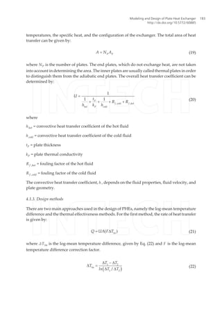
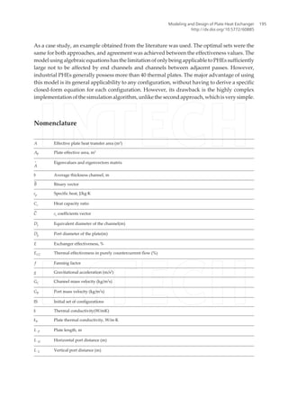
29. also the global optimum. The same optimal set was found with both approaches: two heat
exchanger configurations with 144 channels and a 3-2 asymmetric pass arrangement (as
presented in Table 9).
Boundary conditions
for side I.
Fluid inlet Fluid outlet
For 1 to
0
end
1 1 1
2
Change of pass
for 2 to
for 1 to
1 1
2
1 1 1
2
end
end
Boundary conditions
for side II ( = 1).
Fluid inlet Fluid outlet
for 1 to
0
end
1 1 1
2
Change of pass
for 2 to
for 1 to
1 1
2
1 1 1
2
end
end
Boundary conditions
for side II ( = 2).
Fluid inlet Fluid outlet
for 1 to
1
end
1 1 1
2
Change of pass
for 2 to
for 1 to
1 1
2
1 1 1
2
end
end
Boundary conditions
for side II ( = 3).
Fluid inlet Fluid outlet
for 1 to
0
end
1 1 1
2
Change of pass
for 2 to
for 1 to
1 1
2
1 1 1
2
end
end
Boundary conditions
for side II ( = 4).
Fluid inlet Fluid outlet
for 1 até
1
end
1 1 1
2
Change of pass
for 2 to
for 1 to
1 1
2
1 1 1
2
end
end
Table 6. Boundary conditions [6].
Table 6. Boundary conditions [6].
Heat Transfer Studies and Applications192

30. Table 7. Algorithm to define the flow direction [6].
Side I
for 2 to
for 1 to
2 1 2 1
1
end
end
Side II
for 2 to
for 1 to
2 1 2 1
if = 1: 1
if = 1: 1
if = 1: 1
if = 1: 1
end
end
Table 8. Example data
PLATE CHARACTERISTICS
1.38 m 50 °
0.535 m Φ 1.15
3.7 mm 0.6 mm
150 mm 17 W/m·K
PROCESS-WATER COOLING-WATER
, 87.0 °C , 20.0 °C
26.0 kg/s 62.5 kg/s
CONSTRAINTS
80 150 90%
10 ∆ 20 psi 0 ∆ 25 psi
0.0 m/s 0.6 m/s
It can be seen from the Tables that the simulations using the two models resulted in values that were very close. It is
important to point out that the closed-form equations are only applicable when the end effects can be neglected (in the
present case, when the number of thermal plates was greater than 40).
Table 9. Thermal effectiveness of RS for both mathematical models
#
(differential equation model) (closed-form model)
1 80 1 2 0 80.1 80.3 80.3 80.1 80.4 80.4 80.4 80.4
2 80 2 1 1 80.3 80.1 80.3 80.1 80.4 80.4 80.4 80.4
3 81 1 2 0 80.3 80.3 80.3 80.3 80.6 80.6 80.6 80.6
4 83 2 1 1 80.5 80.5 80.5 80.5 80.8 80.8 80.8 80.8
5 84 1 2 0 80.5 80.8 80.8 80.5 80.9 80.9 80.9 80.9
6 84 2 1 1 80.8 80.5 80.8 80.5 80.9 80.9 80.9 80.9
7 85 1 2 0 80.8 80.8 80.8 80.8 81.0 81.0 81.0 81.0
8 87 2 1 1 80.9 80.9 80.9 80.9 81.2 81.2 81.2 81.2
9 88 1 2 0 80.9 81.2 81.2 80.9 81.3 81.3 81.3 81.3
10 88 2 1 1 81.2 80.9 81.2 80.9 81.3 81.3 81.3 81.3
11 89 1 2 0 81.2 81.2 81.2 81.2 81.4 81.4 81.4 81.4
12 91 2 1 1 81.4 81.4 81.4 81.4 81.6 81.6 81.6 81.6
13 92 1 2 0 81.3 81.6 81.6 81.3 81.7 81.7 81.7 81.7
14 92 2 1 1 81.6 81.3 81.6 81.3 81.7 81.7 81.7 81.7
15 93 1 2 0 81.6 81.6 81.6 81.6 81.8 81.8 81.8 81.8
16 95 2 1 1 81.7 81.7 81.7 81.7 82.0 82.0 82.0 82.0
17 96 1 2 0 81.7 81.9 81.9 81.7 82.1 82.1 82.1 82.1
18 96 2 1 1 81.9 81.7 81.9 81.7 82.1 82.1 82.1 82.1
19 97 1 2 0 81.9 81.9 81.9 81.9 82.2 82.2 82.2 82.2
20 144 2 3 0 71.8 71.7 92.8 92.9 71.8 71.8 93.0 93.0
21 144 3 2 1 71.7 71.8 92.8 92.9 71.8 71.8 93.0 93.0
22 149 3 2 1 71.7 71.7 93.0 93.0 71.7 71.7 93.2 93.2
Optimal configurations
Table 7. Algorithm to define the flow direction [6].
Plate characteristics
L P = 1.38 m β = 50 °
WP = 0.535 m Φ= 1.15
b= 3.7 mm tP = 0.6 mm
DP = 150 mm kP = 17 W/m·K
Process-water Cooling-water
Tin,hot = 87.0 °C Tin,cold = 20.0 °C
M˙
hot = 26.0 kg/s M˙
cold = 62.5 kg/s
Constraints
80 ≤ NC ≤ 150 E min
= 90%
10 ≤ΔPhot ≤ 20 psi 0≤ΔPcold ≤ 25 psi
vhot
min = 0.0 m/s vcold
min = 0.6 m/s
Table 8. Example data
It can be seen from the Tables that the simulations using the two models resulted in values
that were very close. It is important to point out that the closed-form equations are only
applicable when the end effects can be neglected (in the present case, when the number of
thermal plates was greater than 40).
Modeling and Design of Plate Heat Exchanger
http://dx.doi.org/10.5772/60885
193

31. # NC P I
P II Yh
E (differential equation model) E (closed-form model)
ϕ =1 ϕ =2 ϕ =3 ϕ =4 ϕ =1 ϕ =2 ϕ =3 ϕ =4
1 80 1 2 0 80.1 80.3 80.3 80.1 80.4 80.4 80.4 80.4
2 80 2 1 1 80.3 80.1 80.3 80.1 80.4 80.4 80.4 80.4
3 81 1 2 0 80.3 80.3 80.3 80.3 80.6 80.6 80.6 80.6
4 83 2 1 1 80.5 80.5 80.5 80.5 80.8 80.8 80.8 80.8
5 84 1 2 0 80.5 80.8 80.8 80.5 80.9 80.9 80.9 80.9
6 84 2 1 1 80.8 80.5 80.8 80.5 80.9 80.9 80.9 80.9
7 85 1 2 0 80.8 80.8 80.8 80.8 81.0 81.0 81.0 81.0
8 87 2 1 1 80.9 80.9 80.9 80.9 81.2 81.2 81.2 81.2
9 88 1 2 0 80.9 81.2 81.2 80.9 81.3 81.3 81.3 81.3
10 88 2 1 1 81.2 80.9 81.2 80.9 81.3 81.3 81.3 81.3
11 89 1 2 0 81.2 81.2 81.2 81.2 81.4 81.4 81.4 81.4
12 91 2 1 1 81.4 81.4 81.4 81.4 81.6 81.6 81.6 81.6
13 92 1 2 0 81.3 81.6 81.6 81.3 81.7 81.7 81.7 81.7
14 92 2 1 1 81.6 81.3 81.6 81.3 81.7 81.7 81.7 81.7
15 93 1 2 0 81.6 81.6 81.6 81.6 81.8 81.8 81.8 81.8
16 95 2 1 1 81.7 81.7 81.7 81.7 82.0 82.0 82.0 82.0
17 96 1 2 0 81.7 81.9 81.9 81.7 82.1 82.1 82.1 82.1
18 96 2 1 1 81.9 81.7 81.9 81.7 82.1 82.1 82.1 82.1
19 97 1 2 0 81.9 81.9 81.9 81.9 82.2 82.2 82.2 82.2
20 144 2 3 0 71.8 71.7 92.8 92.9 71.8 71.8 93.0 93.0
21 144 3 2 1 71.7 71.8 92.8 92.9 71.8 71.8 93.0 93.0
22 149 3 2 1 71.7 71.7 93.0 93.0 71.7 71.7 93.2 93.2
■ Optimal configurations
Table 9. Thermal effectiveness of RS for both mathematical models
7. Conclusions
In this chapter it was presented the development of two models for the design and optimization
of plate heat exchangers. Both mathematical models were used to accomplish the heat
exchanger design simulations. These methods use differential equations and closed-form
equations based on the notion that a multi-pass PHE can be reduced to an arrangement
consisting of assemblies of single-pass PHEs.
Heat Transfer Studies and Applications194

32. As a case study, an example obtained from the literature was used. The optimal sets were the
same for both approaches, and agreement was achieved between the effectiveness values. The
model using algebraic equations has the limitation of only being applicable to PHEs sufficiently
large not to be affected by end channels and channels between adjacent passes. However,
industrial PHEs generally possess more than 40 thermal plates. The major advantage of using
this model is its general applicability to any configuration, without having to derive a specific
closed-form equation for each configuration. However, its drawback is the highly complex
implementation of the simulation algorithm, unlike the second approach, which is very simple.
Nomenclature
A Effective plate heat transfer area (m2
)
AP Plate effective area, m2
A
= Eigenvalues and eigenvectors matrix
b Average thickness channel, m
B¯ Binary vector
cp Specific heat, J/kg·K
Cr Heat capacity ratio
C¯ ci coefficients vector
De Equivalent diameter of the channel(m)
Dp Port diameter of the plate(m)
E Exchanger effectiveness, %
ECC Thermal effectiveness in purely countercurrent flow (%)
f Fanning factor
g Gravitational acceleration (m/s2
)
GC Channel mass velocity (kg/m2
s)
GP Port mass velocity (kg/m2
s)
IS Initial set of configurations
k Thermal conductivity(W/mK)
kP Plate thermal conductivity, W/m·K
L P Plate length, m
L H Horizontal port distance (m)
L V Vertical port distance (m)
Modeling and Design of Plate Heat Exchanger
http://dx.doi.org/10.5772/60885
195

33. m˙ mass velocity per channel (kg/s)
M˙ Mass flow rate, kg/s
M
= Tri-diagonal matrix
N Number of channels per pass
NC Number of channels
NP Number of plates
NTU Number of transfer units
Nu Nusselt number
OS Optimal set of configurations
P Number of passes
PC Temperature effectiveness
Pr Prandtl number
Q Heat transfer rate(J/s)
R Heat capacity rate ratio
Rf Fouling factor, K/W
Re Reynolds number
RS Reduced set of configurations
si Binary parameter for flow direction
tP Plate thickness, m
U Overall heat transfer coefficient, W/m2
·K
v Fluid velocity inside channels, m/s
WP Plate width, m
Yh Binary parameter for hot fluid location
Yf Binary parameter for type of channel flow
zi Eigenvector of the tri-diagonal matrix
Greek symbols
α Heat transfer coefficient
β Chevron corrugation inclination angle, degrees
ΔP Pressure drop, Pa
ΔTlm Log-mean temperature difference (K)
Heat Transfer Studies and Applications196

34. ΔTM Effective mean temperature difference (K)
η Normalized plate length
θ Dimensionless fluid temperature
λ Eingevalue of the tri-diagonal matrix
μ viscosity (Pa.s)
μw Viscosity at wall temperature (Pa.s)
ρ density (kg/m3
)
Φ Enlargement factor of the plate area
ϕ Parameter for feed connections position
Subscripts
cold Cold fluid
CC Countercurrent
hot Hot fluid
i Generic element
in Inlet
j Generic element
out Outlet
Superscripts
I Odd channels of the heat exchanger
II Even channels of the heat exchanger
max Maximum
min Minimum
Author details
Fábio A.S. Mota1,2
, E.P. Carvalho2
and Mauro A.S.S. Ravagnani2*
*Address all correspondence to: ravag@deq.uem.br
1 National Institute for Space Research, São José dos Campos, SP, Brazil
2 Chemical Engineering Graduate Program - State University of Maringá, Maringá, PR, Brazil
Modeling and Design of Plate Heat Exchanger
http://dx.doi.org/10.5772/60885
197

35. References
[1] Alfa Laval. Canada. Plate Heat Exchanger: A Product Catalogue for Comfort Heating
and Cooling. Available in <http://www. pagincorporated.com>. (Accessed 20 Octo‐
ber 2010).
[2] Sondex. Louisville. Plate Type Heat Exchangers: Operation & Maintenance Manual.
Availble in <http://www.sondex-usa.com>. (Accessed 26April 2011).
[3] Shah, R. K.; Sekulic, D. P. Fundamentals of Heat Exchanger Design. New Jersey: John
Wiley & Sons, Inc. 2003. Page 24.
[4] Taco. Craston. Plate Heat Exchanger: Operational and Maintenance Manual. Availa‐
ble in <http://www. taco-hvac.com>. (Accessed 18 May 2011).
[5] Kakaç S., Liu H., Heat Exchanger: Selection, Rating and Thermal Design, 2ed. Boca
Raton: CRC Press, 2002.
[6] J. A. W. Gut, J. M Pinto, Modeling of Plate Heat Exchangers with Generalized Con‐
figurations. Int. J. Heat Mass Transfer 2003; 46:2571-2585.
[7] Kho, T. Effect of Flow Distribution on Scale Formation in Plate Heat Exchangers.
Thesis (PhD) – University of Surrey, Surrey, UK, 1998.
[8] Wang L., Sundén B., Manglik R. M., Plate Heat Exchangers: Design, Applications and
Performance, Ashurst Lodge: WIT Press, 2007, pp. 27-39.
[9] Alfa Laval. Canada. Plate Heat Exchanger: Operational and Maintenance Manual.
Available in <http://www. schaufcompany.com>. Accessed: 18 May 2011.
[10] Lienhard IV, J. H.; Lienhard V, J. H. A Heat Transfer Textbook. 3ed. Cambridge:
Phlogiston Press, 2004. Page 103.
[11] Kandlikar, S. G.; Shah, R.K. Asymptotic Effectiveness-NTU Formulas for Multipass
Plate Heat Exchangers. Journal of Heat Transfer, v.111, p.314-321, 1989.
[12] Heggs, P. J. e Scheidat, H. J. Thermal Performance of Plate Heat Exchangers with
Flow Maldistribution. Compact Heat Exchangers for Power and Process Industries,
ed. R. K. Shah, T. M. Rudy, J. M. Robertson, e K. M. Hostetler, HTD, vol.201, ASME,
New York, p.621-626, 1996.
[13] Shah, R. K.; Kandlikar, S. G. The Influence of the Number of Thermal Plates on Plate
Heat Exchanger Performance. In: MURTHY, M.V.K. et al. (Ed.) Current Research in
Heat and Mass Transfer. New York: HemisTCPre P.C., 1988, p.227-241.
[14] Kumar, H. The Plate Heat Exchanger: Construction and Design. 1st UK National
Conference of Heat Transfer. n.86, p.1275-1286, 1984.
[15] Gut J. A. W., Pinto J. M, Optimal Configuration Design for Plate Heat Exchangers.
Int. J. Heat Mass Transfer 2004; 47:4833-4848.
Heat Transfer Studies and Applications198

36. [16] Mota F. A. S., Ravagnani M. A. S. S., Carvalho E. P., Optimal Design of Plate Heat
Exchangers. Applied Thermal Enginnering 2014;63:33-39. 2013.
[17] Hewitt, G. F.; Shires, G.L.; Bott, T.R. Process Heat Transfer. Boca Raton: CRC Press,
1994.
[18] Gut, J. A. W.; Configurações Ótimas de Trocadores de Calor a Placas. 2003. 244p.
Tese (Doutorado) – Escola Politécnica, Universidade de São Paulo, São Paulo, 2003.
Modeling and Design of Plate Heat Exchanger
http://dx.doi.org/10.5772/60885
199