This document outlines 23 tutorials on various mathematical topics for students at St. George's College in 2014. It introduces the tutors for the year and describes the structure of the tutorials which will begin with 20-30 minutes of "broad concept problems" followed by 40-60 minutes of help with course-specific work. The broad concept problems are designed to expose students to important mathematical concepts outside the typical curriculum and encourage higher-level thinking. Dimensional analysis and the Buckingham Pi theorem are the topics covered in Tutorial 1, with Tutorial 2 extending these concepts. Subsequent tutorials cover additional topics including differential equations, vector calculus, relativity, and exterior calculus.

![The main idea of the following examples and problems is two-fold: first inspect
an equation and work out the dimensions (or units) of each variable and constant,
given some starting information. We then check whether or not the equation is
dimensionally consistent. Any equation from any area of science and mathematics
must be dimensionally consistent – if it isn’t, then it’s wrong. In this sense, you
don’t need to understand the science or theory behind an equation to deduce when
it is incorrect on dimensional grounds.
4.2 Examples and Problems
Recall lengths, areas and volumes. The fundamental unit that characterizes these
quantities is length: L. Given a rectangular box, with sides of length a, b, c the
volume is VB = a × b × c. Since each of the sides has the dimensions of length:
[a] = [b] = [c] = L, the volume has dimensions
[VB] =[a × b × c]
=[a] + [b] + [c]
=L + L + L
=3L ,
which we interpret as length-cubed: L3. The notation [ ] is used to denote the
dimensions of whatever quantity is inside the brackets. Notice also, that when we
were looking for the dimensions of a product of variables [a × b × c], we added the
dimensions of each variable: [a×b×c] = [a]+[b]+[c] = L+L+L = 3L.Finally,
we ended up with [VB] = 3L, which means that the volume V has 3 factors of the
unit length L – hence volume V has dimensions of length-cubed L3. Of course,
we already knew this!
Similarly to the multiplication rule, if we are inverting quantities we invert their
units – hence: [1
a] = −[a], [ 1
a2 ] = −[a2] = −2[a], etc. Combining this with the
multiplication rule, we get the division rule: [a
b ] = [a] − [b]. For example, if C
is the concentration of protein in milk, it has units ML−3 of mass over volume –
hence dimensionally: [C] = M − 3L.
Exercise 1 Use the rectangular box example to calculate the dimensions of the
area of a rectangle of sides with length ‘a and ‘b , given the area formula
AR = ab. (1)
Now that we have done some simple problems, lets see how dimensional analysis
can be used for error checking. Lets say someone tells us that the volume VS of a
8](https://image.slidesharecdn.com/1f3b3f2a-4e32-4167-891e-7d7de5f1c671-150709175058-lva1-app6892/85/SGC-2014-Mathematical-Sciences-Tutorials-8-320.jpg)
![sphere of radius R is given by
VS =
4
3
πR2
. (2)
Obviously, this is wrong – but if you’ve forgotten the correct formula, there’s an
easy way to see why it is wrong using dimensional analysis. First of all [R] = L,
since radius has dimensions of length. Furthermore, [4
3π] = 0 since this is just a
pure number (so it is dimensionless). Therefore,
[VS] =[
4
3
πR2
]
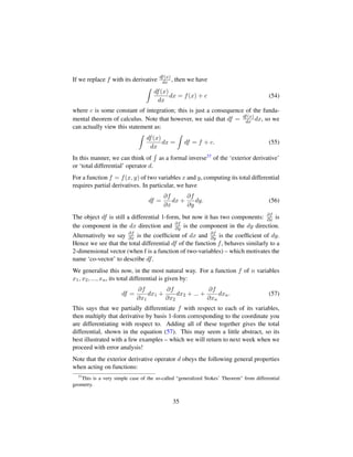
=[
4
3
π] + [R × R]
=[
4
3
π] + [R] + [R]
=0 + L + L
=2L.
But wait a minute, volume has units of length cubed, hence [VS] = 3L. We
then conclude by dimensional arguments that the formula VS = 4
3πR2 is incor-
rect!
Although the last example was easy, the same principles can be applied to much
more complicated formulas in the mathematical sciences – indeed, it is used in
research and in practice when doing estimates, checking articles or performing
large derivations and calculations. Lets do one more example.
Example 1 Newton’s Second Law of Motion: Force = Mass × Acceleration, or
F = ma, is the fundamental postulate governing classical physics between the
late 17th and early 19th centuries. It is vastly important today as the law defines
what the force is, for an object of mass ‘m moving with an acceleration ‘a . The
three fundamental units here are mass M, time T and length L. Displacement ‘x
has dimensions of length L, hence velocity ‘v – which is the rate of change of
9](https://image.slidesharecdn.com/1f3b3f2a-4e32-4167-891e-7d7de5f1c671-150709175058-lva1-app6892/85/SGC-2014-Mathematical-Sciences-Tutorials-9-320.jpg)
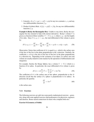
![displacement 3, has units of length over time:
[v] =[
dx
dt
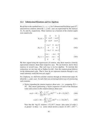
]
=[dx] − [dt]
=[x] − [t]
=L − T , (3)
hence v has units L
T . Similarly, acceleration a is the rate of change of velocity,
hence
[a] =[
dv
dt
]
=[dv] − [dt]
=(L − T) − T
=L − 2T, (4)
which means ‘a has units of length over time-squared: L
T2 . Finally, mass m triv-
ially has units of mass: [m] = M (note that here we use the capital M to denote
the fundamental unit of mass, where as the lower-case m is mass variable that we
insert into Newton’s 2nd Law). Therefore, force F has the following dimensions
[F] =[m][a]
=[m] + [a]
=M + L − 2T,
(5)
whence F has units of (mass × length)/ (time-squared): ML
T2 .
Exercise 2 Use dimensional analysis to conclude which formulas are incorrect on
dimensional grounds – i.e. which of the following formulas are dimensionally
inconsistent. Show your working.
1. A triangle has a base b and a vertical height h, each with dimensions of
length L. Check whether the following formula for its area is dimensionally
consistent
A =
1
2
b2
h. (6)
3
For those of you unfamiliar with the definition of velocity and acceleration in terms of calculus,
you can think of dx
dt
as the change in displacement x over an ‘infinitesimally small amount’ of time
dt. Then dx carries dimensions of length and dt has dimensions of time: [dx] = L , [dt] = T. Note
that in general, for an arbirtrary quantity y, the ‘infinitesimal quantity’ dy carries the dimensions:
[dy] = [y].
10](https://image.slidesharecdn.com/1f3b3f2a-4e32-4167-891e-7d7de5f1c671-150709175058-lva1-app6892/85/SGC-2014-Mathematical-Sciences-Tutorials-10-320.jpg)
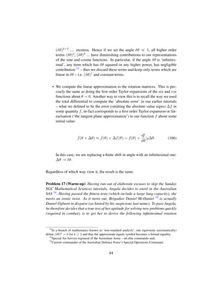
![2. A circle has a radius r with dimensions of length L. Its area is given by
A =
1
2
πr2
. (7)
Is this dimensionally consistent? A stronger question to ask is whether this
formula is correct – if not, why not?
There is one more rule of dimensional analysis which involves analysing equations
which include a sum of terms. In particular, given a quantity A = B + C + D, to
compute the dimensions [A] of A, we don’t just add the dimensions of B, C and
D:
[A] = [B] + [C] + [D], (8)
but rather, we have the consistency requirement that:
[A] = [B] = [C] = [D]. (9)
This is because B, C and D should all separately have the same units. As such,
this observation is very useful for determining the dimension of multiple unknown
quantities in an equation that involves a sum of different terms. For example, the
area of a toddler house drawing is given by: AHouse = ATriangle + ASquare =
1
2bh + a2, where b is the base length of the triangle, h is its vertical length and
a is the length of the sides of the square. Therefore, [AHouse] = [ATriangle] =
[ASquare] = 2L, hence [1
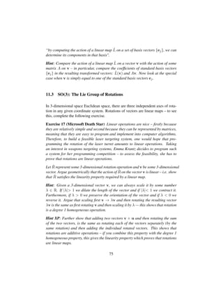
2bh] = [a2] which implies [b] + [h] = 2[a] = 2L.
One last concept: A dimensionless constant, C, is defined to be a quantity which
has no dimensions – hence [C] = 0. These are fundamentally important in the
description of a physical system since they do not depend on the units you choose.
Thus, in some manner they are represent a ‘universal’ quantity or property – indeed,
the dimensionless constants of a system describe a universality class 4.
To answer the following questions, try not to worry too much about terminology
or new and abstract concepts. We are only interested in dimensions – so if you
stay focused and don’t get distracted by the extra information, you can finish them
quickly with no prerequisite knowledge!
Exercise 3 1. A hypercube living in d dimensions has d sides, each with length
a and dimensions of length L. Its hyper-volume has units of Ld and is given
by the formula
V = aD
. (10)
4
A more precise meaning of this statement can be found in the theory of ‘Renormalization
Groups’.
11](https://image.slidesharecdn.com/1f3b3f2a-4e32-4167-891e-7d7de5f1c671-150709175058-lva1-app6892/85/SGC-2014-Mathematical-Sciences-Tutorials-11-320.jpg)
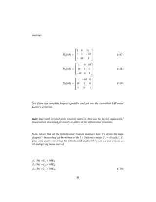
![Verify that this is dimensionally consistent – i.e. show that [V ] = L + ... +
L = d × L. What dimensions would its surface area have? Hint: this would
be same the as dimensions of the area of one of its ‘faces’.
2. The U.S. Navy invests a significant amount of money into acoustic scatter-
ing studies for submarine detection (SONAR). As part of this research, the
Dahlgren Naval Academy uses ‘prolate spheroidal harmonics’ (vibrational
modes of a ‘stretched sphere’) to do fast, accurate scattering calculations. In
this process, a submarine can be approximated to be the shape of a ‘prolate
spheroid’ or ‘rugby ball’. A prolate spheroid is essentially the surface gen-
erated by rotating an ellipse about its major axis. Given a prolate spheroid
with a semi-major axis length a and semi-minor axis of length b, its volume
is
V =
4π
3
ab2
(11)
Is this formula dimensionally-consistent? What about the following formula
for the surface area (it should have units of length-squared):
S = 2πb2
(1 +
a
be
sin−1
(e))? (12)
Note, sin−1
is the ‘inverse sine’ or ‘arcsine’ function. It necessarily pre-
serves dimensionality, hence [sin−1
(e)] = [e]. The variable e is the ‘ec-
centricity’ of the spheroid. It is a dimensionless quantity: [e] = 0, which
measures how ‘stretched’ the spheroid is – i.e. how much it deviates from a
sphere. It is given by the (dimensionally-consistent!) formula:
e2
= 1 −
b2
a2
. (13)
A perfect sphere corresponds to e = 0, where as an infinitely stretched
sphere corresponds to e → 1.
3. In a parallel-universe, Andrew Forrest has a dungeon with BF flawless black
opals inside it. From a financial point of view, these have dimensions of
money $ – i.e. [BF ] = $. A machine recently designed by Ian McArthur,
head of physics at UWA, uses quantum fluctuations of the spacetime vacuum
to produce black opals at a rate of RUWA black opals per minute. Sensing
the loss of his monopoly on the black opal market, Andrew Forrest employs
a competing physicist at Curtin University to create a quantum vacuum sta-
bilizer. This reduces the number of black opals that Ian can produce per
minute by RC black opals per minute, where |RC|≤ RUWA. Working on
12](https://image.slidesharecdn.com/1f3b3f2a-4e32-4167-891e-7d7de5f1c671-150709175058-lva1-app6892/85/SGC-2014-Mathematical-Sciences-Tutorials-12-320.jpg)
![a broad concept problem, a team of first year students at St. George’s col-
lege come up with the following model to predict the value V of shares in
Forrest BlackOps inc. on the stockmarket as a function of time t (time has
dimensions T):
V = β
D
BF
− λ(RUWA + RC)τDe−λ(1− t
τ
)
(14)
where the constant τ (having dimensions of time T) denotes 5 the time at
which European Union is predicted to collapse. Furthermore, D is a function
that measures the market demand for black opals (with no dimensions) and
β is an economic constant predicted by game theory with units of money-
squared: $2. Finally, λ is a dimensionless parameter (so [λ] = 0) that de-
pends on the number of avocados served at the college since the establish-
ment of St. George’s Avocadoes Anonymous up to the given time t.
Is this model dimensionally consistent – i.e. does [V ] = $?
What about the following formula, proposed by students from St. Catherines
College (who didn’t practice dimensional analysis)?
V =
D
BF
− D2
e−t
(15)
On dimensional grounds, list two reasons why this model incorrect.
4. Bonus Question (Don’t worry about the physics, just keep track of dimen-
sions and rules)
The Harvard-Smithsonian Center for Astrophysics is about to release a press-
conference tomorrow (March 17, 2014), indicating the discovery of gravi-
tational waves. Gravitational waves are ripples through spacetime created
by large gravitational disturbances in the cosmos – for example, exploding
stars and coalescing black-holes. These are predicted by Einstein’s theory
of General Relativity – a theory in which gravity is a simple consequence
of the geometry (shape) of spacetime. In this theory, choosing natural units
for the speed of light: c = 1, time and spatial length become dimensionally
equivalent: T = L. Therefore, dimensionally we have: [time] = [distance]
and [c] = [distance/time] = L − T = 0. A geometry which models gravi-
tational waves is described by the following metric (an abstract object which
tells you how gravity and measures of time and length vary at each point in
spacetime):
g = η + h (16)
5
This is the Greek letter tau – not the Roman letter t.
13](https://image.slidesharecdn.com/1f3b3f2a-4e32-4167-891e-7d7de5f1c671-150709175058-lva1-app6892/85/SGC-2014-Mathematical-Sciences-Tutorials-13-320.jpg)
![where η is a flat-space metric (describing an empty universe):
η := −dt + dx ⊗ dx + dy ⊗ dy + dz ⊗ dz (17)
and h is a symmetric-tensor, given in de-Donder gauge by
h := cos(k · r)A +
1
2
× trace(h) × η. (18)
Here is a small (<< 1) dimensionless parameter: [ ] = 0 and A is a sym-
metric tensor field with dimensions of length-squared: [A] = 2L. Note that
the trace operation turns tensors into scalars, so it removes the dimensional-
ity of a tensor: [trace(h)] = 0. Furthermore, consider · as another form of
multiplication. Since the wave vector k and position vector r have inverse
units, we have [k] = −L, [r] = +L – hence [k · r] = 0. For the purposes
of dimensional-analysis, we can treat the tensor product ⊗ as ordinary mul-
tiplication also. The differential quantities have the following dimensions:
[dt] = [dx] = [dy] = [dz] = L, hence [dx ⊗ dx] = 2[dt] = 2L for
example. Since x, y, z, t represent coordinates in spacetime, we also have
[x] = [y] = [z] = [t] = L.
Show that the metric g demonstrates a dimensionally-inconsistent solution
to the Einstein field equations. Where is the error? Suggest what could be
done to this metric to ‘fix’ it and give a dimensionally-consistent solution.
Remark: If you were certain that the equation for h was correct, it would be
unnecessary to tell you the dimensions of A – you could work it out since you
already know [cos(k · r)] = 0 (the function cos(something) is necessarily
dimensionless). Therefore, pretending [A] is unknown, prove that [A] = 2L
given all the other information.
After completing the last two problems, one should realize that much time can be
saved by ignoring most of the information and concentrating only the dimensions
of the variables and constants in the given formulas. This is true in general! There-
fore, to do dimensional analysis, one need not necessarily understand the science
or mathematics behind an equation – but simply the dimensions of the quantities
involved. Therefore, it is an easy way to show when something is wrong without
knowing what you are talking about. 6
6
Dimensional analysis would have saved the present author about 100 hours of supergravity cal-
culations – time which was largely lost due to two dimensionally-inconsistent equations in a pub-
lished journal article.
14](https://image.slidesharecdn.com/1f3b3f2a-4e32-4167-891e-7d7de5f1c671-150709175058-lva1-app6892/85/SGC-2014-Mathematical-Sciences-Tutorials-14-320.jpg)
![4.2.1 Moral of the story
Dimensional analysis can tell you when an equation is wrong, but it doesn’t nec-
essarily imply that an equation is correct – even though its dimensions might be
consistent. As a student, you should make use of dimensional analysis whenever
you can – try it on all formulas you get which have dimensionful quantities. This
will help you to gain a strong intuition of whether or not statements and equations
are sensible and consistent. This helps you to be a fast calculator and it will also
help you to pick up errors in your lecture notes ...
5 Tutorials 2 - Dimensional Analysis and the Buckingham
Pi Theorem (part II)
5.1 Background
One of the key concepts in dimensional analysis is that of dimensionless parame-
ters. Dimensionless parameters are important, because they allow you to charac-
terise both physical and theoretical mathematical systems in a scale-invariant way.
Note that mastering the following concepts and exercises requires a good under-
standing of the material in Tutorial 1. For the more mathematically inclined, one
of the examples and exercises illustrates how to mathematically prove the π theo-
rem by using the rank-nullity theorem from linear algebra – this is a good exercise
for understanding matrix equations and the correspondence between matrices and
simultaneous equations! For the applied minds, we use dimensional analysis to in-
vestigate and form dimensionless constants to characterise the harmonic oscillator,
viscous fluids, electromagnetism and Einstein’s theory of gravity.
BIG DISCLAIMER: Notation
Note that for the most part, we have used ‘additive notation’ to denote the dimen-
sions of some quantity – e.g. [Force] = M + L − 2T. However, in engineering
and sometimes in physics 7, you will often see multiplicative notation being used –
meaning F has dimensions ML
T2 . For these tutorials, we have referred to the later as
the ‘units’ of F, rather than its dimensions. Technically speaking, both are correct
– although units typically refer to some standard of measure, such as kilograms
or kg for the standard SI unit of mass. Here we’ve just taken M, L, T to refer to
both dimensions and their respective standard units. After some practice, it should
7
In particle physics and quantum field theory, additive notation is common for computations as it
is the smarter way to do things.
15](https://image.slidesharecdn.com/1f3b3f2a-4e32-4167-891e-7d7de5f1c671-150709175058-lva1-app6892/85/SGC-2014-Mathematical-Sciences-Tutorials-15-320.jpg)
![3. A set of 3 physical units: mass M, time T, length L (usually kilograms,
seconds, metres).
Now, from these 4 parameters and 3 physical units, I claim that we can form one
dimensionless constant. To do this, one needs to know the dimensions of the pa-
rameters involved. Clearly initial displacement has dimensions of length and initial
velocity has dimensions of length /time: [x0] = L, [v0] = L − T. To work out the
dimensions of the spring constant κ, we inspect the equation of motion.
Since acceleration has dimensions of length over time-squared, we have [d2x
dt2 ] =
L − 2T. Therefore, we have
[m
d2x
dt2
] = [−κx] =⇒
[m] + [
d2x
dt2
] =[κ] + [x]
M + L − 2T =[κ] + L =⇒
[κ] =M − 2T. (21)
Note that the mathematical symbol ‘ =⇒ ’ means ‘implies’. Now that we have the
dimensions of all parameters in this system, we can form a dimensionless product.
In particular, we need one inverse mass factor and two factors of time to cancel the
dimensions in [κ] = M −2T. We can get an inverse unit of mass from [ 1
m ] = −M
and two inverse time units by combining [x0] = L and [v0] = L − T. In particular,
[(x0
v0
)2] = 2[x0] − 2[v0] = 2L − 2(L − T) = 2T. Hence, we get the dimensionless
constant:
G :=
k
m
(
x0
v0
)2
=⇒
[G] =[
k
m
(
x0
v0
)2
]
=[k] − [m] + 2([x0] − 2[v0])
=M − 2T − M + 2T = 0. (22)
Since the constant G has no formal name, we will claim it and call it the ‘Georgian
Constant’ after St. George – the patron saint of dimensional analysis.
The last example illustrated a few important concepts. First of all, we showed
that mathematically all the information about a physical system is giving by a set
of parameters, a set of physical units or dimensions and at least one governing
equation. Second, we showed how we can work the units of an otherwise unknown
constant by using dimensional analysis – this is how we found the dimensions of
the spring constant κ.
17](https://image.slidesharecdn.com/1f3b3f2a-4e32-4167-891e-7d7de5f1c671-150709175058-lva1-app6892/85/SGC-2014-Mathematical-Sciences-Tutorials-17-320.jpg)
![Finally, we showed in this particular case, having 4 parameters and 3 physical
units, we were able to form one dimensionless constant: G . Although we could
have taken any multiple or power of this constant and still arrived at dimensionless
quantity, there essentially only one independent product that we can form out of
the parameters in the simple harmonic oscillator. This is because G, 1
G , G2 or 2G
for example, all contain the same ‘information’.
The last observation is one example of the ‘fundamental theorem of dimensional
analysis’, also known as the ‘π theorem’.
Theorem 1 (Buckingham Pi Theorem) Given a system specified by n indepen-
dent parameters and k different physical units, there are exactly n−k independent
dimensionless constants which can be formed by taking products of the parameters.
Thus in the last example, we saw that the simple harmonic oscillator was described
4 parameters and 3 physical units – hence as claimed, there was indeed only 4−3 =
1 independent dimensionless constant that we could have formed. Hence, any other
dimensionless constant in this system must be some multiple or some power of G.
Before doing the exercises, here is one more example from fluid mechanics.
Example 3 In fluid mechanics, the notion of the ‘thickness’ of a fluid is formalized
by defining its ‘viscosity’. In particular, the dynamic or shear viscosity of a fluid
measures its ability to resist ‘shearing’– an effect where successive layers of the
fluid move in the same direction but with different speeds. For example, relative
to water, glass 10 and honey have a very high shear viscosity, whereas superfluid
Helium has zero viscosity 11.
Given a fluid trapped between two parallel plates–the bottom plate being station-
ary and the top plate moving with velocity v parallel to the stationary plate, the
magnitude of the force required to keep the top plate moving at constant velocity
is given by:
F = ηA
v
y
(23)
Here v is the speed (magnitude of the velocity) of the top plate, A is its surface
area and y is the separation distance between the plate. The parameter η is defined
to be the shear viscosity of the fluid. We can calculate its units using dimensional
analysis. First, from Newton’s 2nd law we know that the force has the dimensions:
[F] = M + L − 2T. Furthermore, the area A has dimensions of length-squared
10
The myth about old church windows sagging is not due to the fact that glass can be modelled as
a viscous liquid, but rather due to the glass-making techniques of past centuries.
11
The transition to the ‘superfluid’ phase occurs below 1 Kelvin – i.e. close to absolute zero
temperature.
18](https://image.slidesharecdn.com/1f3b3f2a-4e32-4167-891e-7d7de5f1c671-150709175058-lva1-app6892/85/SGC-2014-Mathematical-Sciences-Tutorials-18-320.jpg)
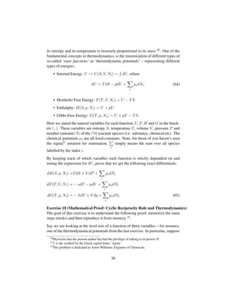
![[A] = 2L, the speed v has dimensions [v] = L − T and the separation y has
dimensions [y] = L. Hence
[F] =[η] + [A] + [v] − [y] =⇒
[η] =[F] − [A] − [v] + [y]
=(M + L − 2T) − 2L − (L − T) + L
=M − L − T (24)
whence η has units of M
LT . Now, the kinematic viscosity ν 12 of the fluid is defined
as the ratio of the dynamic viscosity η and the density ρ (mass per volume) of the
fluid:
ν =
η
ρ
. (25)
Since density has units of mass per length-cubed, we have [ρ] = M − 3L and thus
[ν] = [
η
ρ
] = [η] − [ρ] = M − L − T − (M − 3L) = 2L − T. (26)
In some set of scenarios, we can think of this fluid as parameterized by four pa-
rameters: density ρ, shear viscosity η , kinematic viscosity ν and the fluid speed v
(assuming the fluid only travels in the horizontal direction). Since we have three
different physical units – mass, length and time, the Pi theorem tells us we can
form one independent dimensionless constant. This special, widely-used constant
is called the ‘Reynolds number’ of the fluid and is defined by:
R =
ρvl
η
=
lv
ν
(27)
where l is the ‘characteristic length scale’ for the fluid system (e.g. for a fluid
flowing in a pipe, this length scale would be the diameter of the pipe).
In essence, the Reynolds number expresses the ratio of inertial forces to the viscous
forces. In this manner, it describes relative importance of these two types of forces
in different scenarios. Since it is dimensionless, the Reynolds number is scale
invariant – meaning it characterises the way a fluid will flow on all length scales
(within the valid regime of your theory).
Exercise 4 We defined the Reynolds number R in two ways – one in terms of its
dynamic viscosity η and the other in terms of its kinematic viscosity ν. Show that
the Reynolds number is dimensionless using both of its definitions.
12
This is the Greek letter ‘nu - not the Roman letter ‘v’.
19](https://image.slidesharecdn.com/1f3b3f2a-4e32-4167-891e-7d7de5f1c671-150709175058-lva1-app6892/85/SGC-2014-Mathematical-Sciences-Tutorials-19-320.jpg)
![Example 4 (Mathematical Challenge: Proving the π Theorem) Here is a walk-
through of a proof of the Pi Theorem, using the ‘rank-nullity’ theorem from linear
algebra. For those of you who haven’t encountered matrices before, you can still
make sense of the following in terms of systems of linear equations – but that will
be trickier ... so either save it for later, or talk to your tutor.
Formally, the rank-nullity theorem states that given a m × n matrix (m rows, n
columns) A, which maps n-dimensional vectors to m-dimensional vectors, then
the rank and nullity of the matrix A satisfy:
rank(A) + nullity(A) = n (28)
where the rank of A is defined as the number of linearly independent rows of A
and the nullity of A is defined as the dimension of the kernel of A – i.e. the number
of linearly independent n-dimensional vectors which get mapped to 0 by A. Note
that m ≤ n necessarily (or the system is over-determined).
Now, in the context of dimensional analysis and the π Theorem, we can think a
mathematical or physical system with n parameters and k different types of fun-
damental units (dimensions) as a system of k linear equations in n unknowns, as
follows. Say for example, we have three parameters x, y, z and two fundamental
physical units U1, U2. Then we can represent the dimensions of our parameters
as a matrix by letting each column correspond to different parameters and letting
each row correspond to different fundamental units. So in this example, we let the
first column correspond to the parameter x, the second column to y and the third
column to z. Then the first row corresponds to the unit U1 second row to the unit
U2. Then the entry in the first row and column corresponds to the number of di-
mensions of x has in the unit U1. So if for example, x has the units Ua
1 Ub
2 then it
has dimensions: [x] = [Ua
1 ] + [Ub
2] = aU1 + bU2. Similarly, let y have units Uc
1Ud
2
and z have units Ue
1 Uf
2 : hence [y] = cU1 + dU2 and [z] = eU1 + fU2. We can
form the ‘dimensional matrix’ D for this physical system, which is represented as:
D =
a c e
b d f
(29)
To see that this makes sense, we can simply act13 the transpose of the dimensional
matrix DT on the vector U =
U1
U2
containing the physical units to recover all
three of our dimensional equations [x] = aU1 + bU2, [y] = cU1 + dU2 etc. To find
dimensionless constants, we have to solve the ‘nullspace equation’:
13
By matrix multiplication.
20](https://image.slidesharecdn.com/1f3b3f2a-4e32-4167-891e-7d7de5f1c671-150709175058-lva1-app6892/85/SGC-2014-Mathematical-Sciences-Tutorials-20-320.jpg)
![QI:Using Newton’s 2nd Law, F = ma, deduce the dimensions or units of GN .
Note that you are working with mass, length and time (M,L,T) as your fundamental
units, hence [m1] = [m2] = M. Furthermore, by definition the unit vector 16
ˆr = r2−r1
|r2−r1| is dimensionless: [ˆr] = 0. Note that in general, the dimensions or
units of a vector quantity are always the same as the units of the magnitude (and
components) of that vector – hence [r] = [r] for example.
Now that we have the dimensions of GN , we are ready to consider Einstein’s theory
of gravitation. Einstein’s theory differs from Newton’s theory in many ways – fun-
damentally it explains gravity as a consequence of spacetime curving around any
object with mass, where the ‘amount’ of curvature being greater for greater masses
(e.g. the Sun). On an astrophysical level, it is important as it helps to explain the
big bang, solar fusion and the existence of the black holes – objects which are nec-
essary for the stability of some galaxies such as the Milk Way. In terms of everyday
living, general relativity is essential for the operation of GPS satellites – without
the gravitational corrections to the timing (gravitational time-dilation) offered by
Einstein’s theory, the GPS system would not be accurate enough to work.
In Einstein’s theory, spacetime is modelled by the following objects 17
• A energy-momentum tensor T which contains information about ‘sources’
of curvature – matter and energy. It’s components have dimensions of an
energy-density: [Tab] = [ Energy
V olume ] = M − L − 2T. Since the tensor itself is
a second-rank covariant tensor, we have: [T] = [Tabdxa ⊗ dxb] = [Tab] +
[dxa ⊗ dxb] = M − L − 2T + 2L = M + L − 2T.
Note that the dimensionality of energy can be deduced from the relation:
Work = Force × Distance and hence [Energy] = [Work] = [Force] +
[Distance] = M + L − 2T + L = M + 2L − 2T.
• A metric tensor g describing how gravity distorts measures of length and
time. This has units of length-squared: [g] = 2L.
• The Riemann Curvature tensor, Riem, describes how the curvature of space-
time varies in different regions. It also measures how gravity distorts parallel-
16
Here r1 and r2 are the position vectors describing the location of the masses m1 and m2 with
respect to some origin.
17
Note that most physicists do not understand differential geometry, hence when they speak of ten-
sors they usually are talking about components of tensors. This won’t matter here, but for reference,
if you ever want to compare: covariant tensors have two extra factors of length compared to their
components and contravariant tensor have two factors less than their components – which basically
means adding ±2L to the dimensions.
24](https://image.slidesharecdn.com/1f3b3f2a-4e32-4167-891e-7d7de5f1c671-150709175058-lva1-app6892/85/SGC-2014-Mathematical-Sciences-Tutorials-24-320.jpg)
![transport. It is given roughly 18 as the anti-symmetrized second tensor ‘gra-
dient’ of the metric: Riem ∼ ⊗ ⊗ g, where are a type of derivative
operator and ⊗ is a type of multiplication for tensors.
• The Ricci tensor, Ric, is given by taking the trace of the Riemann tensor:
Ric = Trace(Riem). It describes how gravity distorts volumes and is also
related to how different geometries evolve under the heat equation.
• The Ricci Scalar R – this quantity is a function which measures how gravity
locally distorts volumes. Einstein’s theory can be derived by saying that
nature minimizes this quantity – an approach due to a mathematician named
David Hilbert 19. It is given by the taking the trace of Riemann tensor twice:
R = Trace(Trace(Riem)) = Trace(Ric).
• The speed of light, c. This universal speed limit quantifies how fast mass-
less particles can move and also how fast gravitational disturbances (gravity
waves) can propagate. It has dimensions of speed: [c] = L − T.
QII:Using the above information, derive the dimensions of Newton’s gravitational
constant GN again, this time using Einstein’s law of gravity:
Ric −
1
2
Rg =
8πGN
c4
T. (32)
You will need the following facts: the derivative operator reduces the length
dimension of a tensor by one factor, whereas the tensor product ⊗ raises it by one
factor (in this case). Hence [Riem] = 2[ ] + 2[⊗] + [g] = −2L + 2L + 2L = 2L.
Furthermore, the trace of a (covariant) tensor reduces its length dimension by two
factors, hence for example: Trace[Riem] = [Riem] − 2L.
Tip: To ease calculations, you may use so-called ‘natural units’ where the speed
of light c = 1. In these units length and time have the same dimensionality, hence
[c] = [Distance] − [Time] = 0 and T = L. You will then get the dimensions of
GN in natural units which you can compare to your value of GN using Newton’s
Law, after you set T = L.
Finally, we are in a position to understand a very special dimensionless constant –
the ‘gravitational coupling constant’, αG. Since it is dimensionless, this constant
characterises the strength of the gravitational force on all length scales (within the
regime of validity of Einstein’s theory). It can be defined in terms of any pair of
stable elementary particles – in practice, we use the electron.
18
Don’t ever show this to a differential geometer. If you want the real definition, see me.
19
In retrospect, David Hilbert deserves almost the same level of credit as Einstein for the theory
of general relativity.
25](https://image.slidesharecdn.com/1f3b3f2a-4e32-4167-891e-7d7de5f1c671-150709175058-lva1-app6892/85/SGC-2014-Mathematical-Sciences-Tutorials-25-320.jpg)
![In particular, we have:
αG =
GN m2
e
¯hc
≈ 1.7518 × 10−45
(33)
where c is the speed of light, GN is Newton’s gravitational constant and me is the
mass on an electron. The quantity ¯h = h
2π is the reduced Planck constant which
characterises the scale at which matter exhibits quantum behaviour such as wave-
particle duality 20
QIII:Show that the gravitational coupling constant αG is indeed dimensionless.
Note that [me] = M. To work out the dimensions of ¯h = h
2π , you will need the
Planck-Einstein relation which relates the energy of a photon (particle of light) its
frequency:
E = hf. (34)
Then [h] = [E] − [f]. Since the frequency of light is the number of oscillations
of the electromagnetic wave per unit time, we have [f] = −T. You can get the
dimensions , [E] of energy E from the calculation shown above for the energy-
momentum tensor.
Now, for the last part of this problem, we introduce one more fundamental phys-
ical unit: the unit of electric charge, Q 21. Similar to the gravitational coupling
constant, there is a dimensionless constant which characterises the strength of the
electromagnetic interaction (which is responsible for almost all of chemistry) – the
‘fine structure constant’ αEM . The value of this constant is (accurately) predicted
and measured using the theory of Quantum Electrodynamics, which is a type of
quantum field theory largely due to Richard Feynmann and Freeman Dyson. It is
given by
αEM =
1
4π 0
e2
¯hc
(35)
where 0 is electric permittivity of the vacuum. It has units [ 0] = [Farads/Meter] =
[Seconds4 Amps2 Meters−2 kg−1] = 4T + 2Q − 2T − 2L − M. Hence
[ 0] = 2T + 2Q − 2L − M. The parameter e is the charge of an electron, with
dimensions [e] = Q.
Using ‘natural units’ – a popular convention in particle physics, we set all of our
previous parameters to equal 1. Thus, 4πGN = c = ¯h = 0 = 1, where 0 is
20
If ¯h was really large – say ¯h ≈ 1 for example, then we would observe wave-particle duality on
a macroscopic scale and the universe would be a scary, crazy place. Bullets would diffract through
doorways and Leanora’s fists could quantum tunnel through walls.
21
The SI unit for charge is Coulombs.
26](https://image.slidesharecdn.com/1f3b3f2a-4e32-4167-891e-7d7de5f1c671-150709175058-lva1-app6892/85/SGC-2014-Mathematical-Sciences-Tutorials-26-320.jpg)
![24. In these models, the extra-dimensions take the form of some compact hypersur-
face. Newton’s gravitational constant GN is then theoretically explained using the
formula 25:
GN =
3κ2
16πS
(38)
where S is the surface-area of the extra dimensions and κ is Einstein’s constant,
with dimensions [κ] = [GN ].
QV:The above formula for GN is correct, even though it may look dimensionally
incorrect. What units would S need to have for dimensional consistency? In that
case, what quantity does the surface-area S actually represent? Hint: Recall the
‘unit vector’ in Newton’s law of gravity.
The last problem illustrates a common theme in engineering, physics and math-
ematics – normalization. Normalized quantities are typically dimensionless! As
such, they are very useful and friendly to work with.
24
Supersymmetry removes the problem of Tachyons in String Theory and also stabilizes the mass
of the Higgs boson.
25
First derived in this generality by the present author in 2013.
28](https://image.slidesharecdn.com/1f3b3f2a-4e32-4167-891e-7d7de5f1c671-150709175058-lva1-app6892/85/SGC-2014-Mathematical-Sciences-Tutorials-28-320.jpg)
![1. Given a circular cylinder of radius r and height h, we can view its volume V
and surface area S as functions of two variables:
V (r, h) =πr2
h
S(r, h) =2π(r2
+ rh). (61)
Compute the exterior derivatives dV and dS.
2. An elliptical cylinder is a cylinder with elliptical cross-sections – you can
think of its as ellipses stacked on top of each other ... 38 Given an elliptical
cylinder with height h, cross-sectional ellipses with semi-major axes lengths
a and semi-minor axes lengths b, its volume V and surface area S can be
viewed as functions of three variables
V (a, b, h) =πabh
S(a, b, h) =2πab + 2πph. (62)
where p is the perimeter of the elliptical cross-sections. To express p exactly,
one requires an infinite series:
p = 2πa(1 −
∞
n=1
(2n)!2
(2nn! )4
e2n
2n − 1
) (63)
where e =
?a2−b2
a is the eccentricity of the ellipse. Using the Ramanujan39
approximation: p ≈ π[3(a+b)−
—
(3a + b)(a + 3b)], compute the exterior
derivatives dV and dS.
3. For those of you who have studied infinite series, compute dS using the exact
expression for the perimeter of an ellipse stated above.
Given these examples, in addition to the previous exercises, complete the following
problems.
Exercise 9 (Exact Differentials: Thermodynamics/Thermochemistry) Thermodynamics
is a broad theory, originally explaining the phenomenon that we know as ‘heat’.
More generally, it governs a vast range of macroscopic phenomena in nature –
from reaction rates in thermochemical processes to the surface area of blackholes.
The most famous abstraction of thermodynamics, due to Steven Hawking, Bill Un-
ruh and Jacob Bekenstein, is that the surface area of a black hole is proportional to
38
Puns – bringing English lit and mathematics together since 1600.
39
A famous Indian child prodigy and mathematical genius who made great rediscoveries and con-
tributions to number theory, estimations and analysis in isolation.
37](https://image.slidesharecdn.com/1f3b3f2a-4e32-4167-891e-7d7de5f1c671-150709175058-lva1-app6892/85/SGC-2014-Mathematical-Sciences-Tutorials-37-320.jpg)
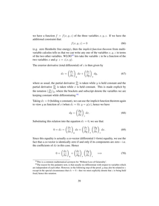
![• A mathematical function relating your derived quantity to the quantities you
directly measure.
• The ‘total differential / exterior-derivative / exact derivative’ formula (Tuto-
rial 4).
Mathematically, we proceed as follows.
Definition 1 (Absolute Error) Let x1, ..., xn be a set of n quantities which are
to be measured (with their respective units). Now, let f(x1, ..., xn) be a func-
tion of n variables, representing some derived quantity which is to be measured.
If ∆x1, ..., ∆xn are the errors associated to the measurements of x1, ..., xn (e.g.
instrument precision) then the corresponding ‘absolute error’ in f(x1, ..., xn) is
given by the linear estimate:
∆f(x1, ..., xn) = |
∂f
∂x1
∆x1|+|
∂f
∂x2
∆x2|+... + |
∂f
∂xn
∆xn|. (74)
which is evaluated at the measured values x1, ..., xn.
Note that the formula for ∆f is similar to the total differential, df, where the dif-
ference is that we have replaced the covectors (1-forms) dx1, ..., dxn with the mea-
surement errors ∆x1, ..., ∆xn. The absolute value of each term is also taken – this
is because when looking to estimate the ‘Maximum Probable Error’, each error
should add up. When quoting the value of f as (derived) measurement, we say that
the quantity f has the value:
Measured Value of f = f(x1, ..., xn) ± ∆f. (75)
Therefore, (with some probability) we say that the true value of f lies in the interval
[f − ∆f, f + ∆f].
Note that in the case of perfect measurement technique, one would attribute the
errors ∆x1, ..., ∆xn to the instrumental precision. So for example, if you are mea-
suring the height h of Tyrion Lannister with a tape measure, the error ∆h would be
equal to half the width of the gradings in the tape measure. Finally, one should note
that this ‘absolute error’ formula only takes deterministic errors into account (i.e.
precision e.t.c) – it does not factor in wrong measurement technique or external
errors which one has not accounted for.
Before attempting the problems and examples, consider the following philosoph-
ical note. Because of Quantum Mechanics – in particular, the Heisenberg Un-
certainty Principle and the inherent non-deterministic nature of the universe, it is
inherently impossible to measure anything with 100% accuracy or certainty. This is
42](https://image.slidesharecdn.com/1f3b3f2a-4e32-4167-891e-7d7de5f1c671-150709175058-lva1-app6892/85/SGC-2014-Mathematical-Sciences-Tutorials-42-320.jpg)
![Hint: To proceed, you should write the volume V in terms of the circular and
elliptical circumferences: V = V (CC, CE). This requires writing the semi-minor
and semi-major axis lengths in terms of the Circumferences. We already know that
b = R, hence b = CC
2π . To get the semi-major length a in terms of CE, one needs
an approximation for the elliptical integral E(e). Recalling from Russian Grade 1
in Tutorial 4, we have the Ramanujan approximation:
CE ≈ π[3(a + b) −
—
10ab + 3(a2 + b2)]. (83)
By bringing the 3(a + b) term to the left-hand side and squaring both sides, we can
obtain a quadratic equation for a in terms of b and CE. The positive root of this
equation is given by:
a =
3CE − 4bπ +
˜
3C2
E + 12bCEπ − 20b2π2
6π
. (84)
Substituting these expressions for a and b into V , one can then compute V and its
partial derivatives, required for computing ∆V .
Exercise 13 (La forma de la espada – “The Shape of the Sword”) The goal of
this problem, is to be able to reproduce all the steps and arguments to derive the
volume estimate – then compute the volume measurement and absolute error at the
end. Disclaimer: there may be errors in this error analysis!
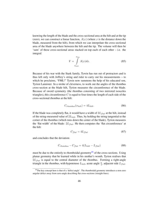
To add further insult to the Stark family, Tywin Lannister – Hand of the King
and head of the Lannister family, decides to melt down Edard Stark’s greatsword,
“Ice. Being a pragmatic man, Tywin decides to calculate the volume of this sword
in order to work out how much Valyrian steel he will have to forge two new swords,
for his sons.
Not being as clever as Archimedes, Tywin doesn’t think to use water displacement
to measure this volume. Instead he proceeds as follows. We can approximate the
blade (Valyrian steel part) of the sword to be that of a shallow rhomboidal prism,
with maximum width at the hilt of the sword, decreasing in thickness down to the
pointed tip. A rhomboidal (diamond-shaped) prism, means that the width-wise
cross-sections of the sword of are shaped like rhombuses with very narrow (acute)
angles α in the plane parallel to the cutting edges and very large (obtuse) angles
β length in the plane perpendicular to the cutting edge. Despite the decreasing
thickness, the angles in the rhombus cross-sections will remain the same48.
Say that the rhomboidal cross-sections are measured to linearly decrease in area,
down from the hilt to the tip – reached zero area at the pointed end of the blade. By
48
So we could in-fact view the blade as a continuous conformal map of a rhombus.
45](https://image.slidesharecdn.com/1f3b3f2a-4e32-4167-891e-7d7de5f1c671-150709175058-lva1-app6892/85/SGC-2014-Mathematical-Sciences-Tutorials-45-320.jpg)
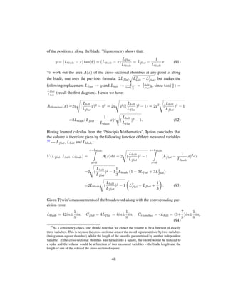
![Figure 1: Cross-sectional rhombus of idealized broadsword.
Therefore, simple trigonometry gives:
cos(
α
2
) =
Lflat
Lhilt
sin(
β
2
) =
Lflat
Lhilt
, (89)
which allows Tyrion to deduce the interior angles α and β of the cross-sectional
rhombus. By symmetry, the area of the cross-sectional rhombus at the hilt is simply
four times the area of this triangle (using Pythagoras’ theorem since we want all
quantities in terms of the measured quantities Lh, Lf )
Arhombus(xhilt) =4 ×
1
2
× base × height = 4 ×
1
2
Lflat
˜
L2
hilt − L2
flat
=2Lflat
˜
L2
hilt − L2
flat . (90)
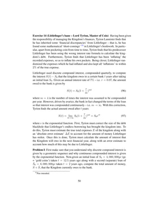
To work out A(x) for any x ∈ [xhilt, xtip], Tyrion lays the sword flat. Overhead, the
sword looks like an isosceles triangle, with base 2Lflat and height Lblade. Splitting
these into two right-angled triangles, we get the following diagram:
Figure 2: Top view of broadsword laid flat.
In particular, Tyrion finds that tan(γ) =
Lflat
Lblade
. Setting up a coordinate system
with xhilt := 0 at the hilt and x = xtip = Lblade at the end of the blade, the height
y of the triangle at any point along the blade, can then be computed as a function
47](https://image.slidesharecdn.com/1f3b3f2a-4e32-4167-891e-7d7de5f1c671-150709175058-lva1-app6892/85/SGC-2014-Mathematical-Sciences-Tutorials-47-320.jpg)
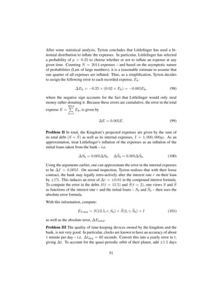
![one can deduce the following measurements and (reduced) errors for the L vari-
ables 51
Lblade = [42 ±
1
8
] in, Lflat = [1 ±
1
2
] in, Lhilt = [
1
4
(3 +
7
8
) ±
1
2
] in. (95)
Problem I From these measurements, compute the volume (in units of inches
cubed), V , of Ned’s broadswoard along with the corresponding absolute error, ∆V .
Convert these measurements into metric units, using the conversion: 1 inch =
2.54 cm.
In a thoughtful moment, Tyrion decides to calculate the financial worth of the
sword in terms of pure Valyrian steel. Given that Valyrian steel is worth 100
times its weight in gold, calculate the total worth W of the broadsword in terms
of kilograms of gold. To do this, use the fact that density of Valyrian steel 52 is
ρ = 7.85 g/cm3 = 0.284 lb/in3. Remember to use consistent units – either stick
with imperial units or convert everything to metric units.
Problem II Given that mass M = V olume × Density = V ρ, compute the
error in the amount of gold Tyrion will make by selling the steel smelted from
the broadsword blade. Assume that the density ρ given is accurate to the num-
ber of decimal places quoted – i.e. the precision error in density is given by:
∆ρ = 0.005g/cm3. Hence deduce the minimum and maximum amount of gold
(W = 100M) Tyrion will make, based on Tywin’s measurements – i.e. compute
W − ∆W and W + ∆W.
• The dimensions in the last question were computed using slightly larger-
than-average dimensions for Claymores and Two-handed swords from the
medieval ages.
• The last exercise illustrates an important technique in making measurements:
by measuring the circumference of the sword rather than just the edge of
the cross-sectional rhombus, the precision error in determining Lflat was
reduced by a factor of 4. In general when making measurements, it is better
to make measurements of quantities which are much larger than the precision
limitation set by your instrument – from these measurements, you can then
deduce measurements for quantities you need with lower precision error. So
for example, in determining the area of a circle with string, it is better to
measure its circumference rather than its radius (since the former is larger) –
this way, one may reduce the precision error in determining the radius by a
factor of 2π.
51
See the remark after this exercise.
52
The density of Carbon 1060 Steel used to make “Ice” replicas for crazy Game of Thrones fans.
49](https://image.slidesharecdn.com/1f3b3f2a-4e32-4167-891e-7d7de5f1c671-150709175058-lva1-app6892/85/SGC-2014-Mathematical-Sciences-Tutorials-49-320.jpg)
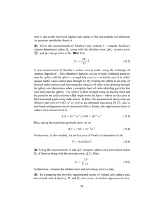
![(oops!). Snorlax suspects she may in fact have cancer, so decides to consult Dr.
Kaylin Hooper – another Georgian medical student. Dr. Hooper suggests that one
way to test for cancer, is to measure Snorlax’s average density and compare this
density to that of a healthy sphere – since sentient sphere’s don’t have muscles or
bone or any internal structure ... the standard deviation in sphere densities amongst
the sphere population is extremely small. Having learned that type 1 spherical
cancer tumors have a higher density than that of healthy sphere tissue and type 2
tumors have a lower density than that of normal tissue, Dr. Hooper proposes that if
Snorlax’s density is significantly higher or lower than the sentient sphere average
density (to within 5 standard deviations and experimental error), then Snorlax has
sphere cancer.
Using Nuclear Magnetic Resonance Imaging (MRI = NMR) and a reconstruction
algorithm based on Ellipsoidal Harmonics (http://www.sciencedirect.
com/science/article/pii/S0010465513002610), Dr. Hooper mea-
sures Snorlax’s volumetric density to be:
ρexp = 103
kg/m3
, (109)
with a combined least-scale and numerical precision error (inherent in the algo-
rithm) of
∆ρexp = 0.001g/m3
. (110)
Pro Tip: Remember to keep track of the units you use and be consistent (e.g.
choose kilograms and metres).
Q0: A standard healthy sentient sphere has a density of ρavg = 969kg/m3 with a
population standard deviation of σρ = 6kg/m3. Using the particle physics stan-
dard of ‘5-sigma’ for statistical significance, determine whether or not Snorlax has
sphere cancer. If so, what type of sphere cancer(s) does Snorlax likely have?
In other words, does the possible range of Snorlax’s experimentally measured den-
sity, [ρexp − ∆ρexp, ρexp + ∆ρexp] lie entirely within the density of the standard
sphere population ρavg = 969kg/m3, to within 5 standard deviations, 5σρ –i.e.
[ρavg − 5σρ, ρavg + 5σρ]?
Furthermore, compute the relative error and percentage error in the experimentally
determined value of Snorlax’s density.
Q1: As an upcoming student in medicine, Matthew Fernandez realises that setting
the statistical significance level to five standard deviations is crazy for a medical
diagnosis. After some research, Matthew decides that setting a significance level of
three standard deviations to diagnose for sphere cancer, is far more sensible. Under
56](https://image.slidesharecdn.com/1f3b3f2a-4e32-4167-891e-7d7de5f1c671-150709175058-lva1-app6892/85/SGC-2014-Mathematical-Sciences-Tutorials-56-320.jpg)
![whether or not Snorlax has volumetosis. If Snorlax has volumetosis, how severe is
it – i.e.
Hint: This amounts to comparing whether or not the measurement ranges, [Rv −
∆Rv, Rv +∆Rv] and [Rs −∆Rs, ∆Rs +∆Rs], overlap or not. The severity is de-
termined by the ‘range of disagreement’ – i.e. the maximum possible discrepancy
(non-overlap).
Q6 Type I volumetosis and Type II volumetosis can be distinguished as follows. In
particular, for some currently unknown reason, Type I volumetosis typically leads
to a sphere turning into a slightly oblate spheroid, meaning that its surface area
increases relative to its volume. This is because for a given volume, a sphere is an
object which has minimum surface area. Hence, in Type I volumetosis, the sur-
face area determined radius Rs of Snorlax would be measured to be consistently
greater than Snorlax’s volume-determined radius Rv. Since this form of volume-
tosis is topological, it can be treated by injecting Snorlax with ‘homeomorphism’
regulators which then continuously transform Snorlax’s gene expression back to
that of zero eccentricity.
In the case of Type II volumetosis, because the quantum superpositions are sym-
metrically weighted about some classical radius, on average (i.e. after a large num-
ber of measurements), the volume and surface area determined radii agree. How-
ever, because of the oblate spheroid mystery, it suffices to measure whether or not
the Rv is greater than Rs. In particular, if Rs Rv, Snorlax has Type II volumeto-
sis, which cannot be cured by Dr. Punch or Dr. Hooper – for this, the Royal Perth
Hospital must bring in an external contractor, known as Dr. Who. Such an affair, is
extremely expensive.
From this, decide whether or not Snorlax requires the medical attention of Dr.
Who.
59](https://image.slidesharecdn.com/1f3b3f2a-4e32-4167-891e-7d7de5f1c671-150709175058-lva1-app6892/85/SGC-2014-Mathematical-Sciences-Tutorials-59-320.jpg)
![Problem 12 (Easy Proof) Using the previous formula (146), prove that u×v = 0
whenever u and v are parallel.
Furthermore, argue geometrically on the basis of the previous formula (146), why
u · (u × v) = 0.
You may recognize that the quantity u × v given by the formula (146) is simply
the area of a parallelogram with sides u and v.
Problem 13 Given vectors v and u with units of length: [v] = [u] = L, use
dimensional analysis and formula (146) to show that their cross product has units
of area, L2.
It may seem strange that the cross-product produces a vector with different units to
each of the vectors you are crossing – however, this is natural when you consider
the applications of the cross-product to physics and engineering. More importantly,
it relates to the fact that the cross product is in-fact a ‘pseudovector’ rather than a
true vector – a concept which is only properly understood in the context of a more
general product called the ‘exterior product’ and an operation called the ‘hodge
dual’. You can however, think of a pseudo-vector as one which behaves like a
vector when rotated, but reverses direction (changes sign) when reflected.
Problem 14 (Simple Calculations) Using the area formula for the cross product,
compute areas of the parallelograms formed by the following sets of vectors in
three dimensions:
• e1 and e2
• e1 and e3
• e2 and e3.
Finally, we finish on a rather important set of identities.
Problem 15 (The Rotation Algebra: so(3)) Using the properties of the cross-product
listed in this tutorial (or otherwise), prove the following critical identities for the
standard Cartesian basis vectors in three dimensions:
• e1 × e2 = e3
• e2 × e3 = e1
• e3 × e1 = e2.
Hint: It suffices to show that (ej × ek) = ijkei.
71](https://image.slidesharecdn.com/1f3b3f2a-4e32-4167-891e-7d7de5f1c671-150709175058-lva1-app6892/85/SGC-2014-Mathematical-Sciences-Tutorials-71-320.jpg)
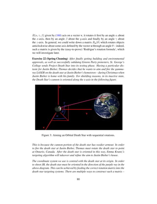
![the rotation ˆR with respect to the rotation angle δθ, is given by:
δv
δθ
=
( ˆR(δθ) − I3)
δθ
v. (176)
This looks suspiciously like a derivative – it is in fact a formal derivative if we
take the limit as the rotation angle δθ → 0. To see this, we consider a vector
u(θ) which is a function of the rotation angle θ performed by the rotation ˆR(θ). In
particular, we let this vector function coincide with the constant vector v when it
is not-rotated – i.e. u(θ = 0) = v. For a general rotation angle θ, we therefore
have u(θ) = ˆR(θ)u. The infinitesimal rate of change of this vector function with
respect to θ is therefore expressed as the derivative:
d
dθ
u(θ) = [
d
dθ
( ˆR(θ) − I3)]v = [
d
dθ
ˆR(θ)]v. (177)
We take the derivative of a matrix which has functions as entries by taking the
derivative of each function – since the identity matrix I3 is constant, its derivative
is just the zero matrix: d
dθ I3 = 0. Since we were considering infinitesimal rotations
originally (‘small angles close to zero’), we evaluate this derivative of the vector
function u(θ) at the origin θ = 0 (which means taking the derivative then setting
θ = 0):
d
dθ
u(θ)|θ=0= [
d
dθ
( ˆR(θ)]|θ=0v. (178)
Notice that as θ varies, the vector u(θ) traces out a curve78 as it rotates – since the
vector d
dθ u(θ)|θ=α represents the rate of change of u at θ = α, is therefore tangent
to the curve at θ = α. Equivalently, we can consider the derivative of the rotation
matrix [ d
dθ ( ˆR(θ)]|θ=α to be ‘tangent to the rotation operator’ ˆR(θ) at θ = α in
the abstract sense. When θ = 0, any rotation operator is simply represented by
the identity matrix I3 – which is the identity element of the Lie Group SO(3) of
rotations 79. Hence infinitesimal rotations correspond to rotation matrices which
are ‘close’80 to the identity matrix I3.
As it turns out, if we restrict our attention to the behaviour of the rotation group
SO(3) about the origin – i.e. infinitesimal rotations and rotation matrices ‘close’
to the identity matrix I3, then in particular, the matrices:
d
dθ
ˆR(θ)|θ=0 (179)
78
Such curves are called ‘integral curves’ and the vector field d
dθ
u(θ) corresponds to the ‘direction
fields’ you may know from the theory of differential equations.
79
Recall the last tutorial
80
The notion of matrices being ‘close’ can be formalized by defining a metric or ‘norm’ (notion
of distance) for matrices – for example, the Froebenius or Hilbert-Schmidt operator norms.
87](https://image.slidesharecdn.com/1f3b3f2a-4e32-4167-891e-7d7de5f1c671-150709175058-lva1-app6892/85/SGC-2014-Mathematical-Sciences-Tutorials-87-320.jpg)
![Definition 8 A Lie algebra g is a vector space83 g (over a field F) equipped with a
binary operation84
[ , ] : g × g → g
(u, v) → [u, v] (181)
called the ‘Lie bracket’, which satisfies the following properties:
1. Left Linearity:
[αu + βv, w] = α[u, w] + β[v, w] ∀u, v ∈ g, ∀α, β ∈ F (182)
2. Anti-symmetry:
[u, v] = −[v, u] ∀u, v ∈ g, ∀α, β ∈ F (183)
3. Jacobi Identity:
[u, [v, w]] + [v, [w, u]] + [w, [u, v]] = 0 ∀ u, v, w ∈ g. (184)
Thus, we can think of a Lie algebra as a vector space whose vector multiplication
operation is the Lie bracket. However, earlier we said that the tangent matrices
{Ej} were elements of the Lie algebra – implying that they are vectors. This is not
a mistake – when we refer to a Lie algebra g as a vector space, it means a vector
space in an abstract sense (not column vectors!). A quick review of the vector
space axioms85 (defining properties) should reveal that the set of n × n real or
complex-valued matrices form a vector space – the basis for the vector space has
n2 basis vectors; one such basis consists of the matrices µij whose entries are all
zero except for entry in the i − th row and j − th column (which we can set to
be 1). In this manner, what we referred to as ‘tangent matrices’ are indeed tangent
vectors in this abstract sense.
Problem 20 (The Girl Who Cried Wolf) In one of many universes in the multi-
verse, a St. George’s fresher by the name of Sophia Lie continually makes excuses
not to attend the SGC Mathematical Sciences tutorials. This is because she has
questioniaphobia – a fear of asking questions. One day, an optically- and radar-
cloaked spaceshuttle docks with the the St. George’s College Dragon (the newly
83
Recall that a vector space over a field F is a set of vectors which obey the usual rules of vector
addition and scalar multiplication – for our purposes we usually take the field to be the real or
complex numbers, R and C.
84
Recall we defined binary operations in Tutorial 8.
85
Ask your tutor.
89](https://image.slidesharecdn.com/1f3b3f2a-4e32-4167-891e-7d7de5f1c671-150709175058-lva1-app6892/85/SGC-2014-Mathematical-Sciences-Tutorials-89-320.jpg)
![elected name for the Death Star). A team of Saint Catherine’s raiders board the
shuttle and capture Sophia while she is in her room – destroying the Dragon’s fine-
targeting systems on the way. Sophia sends an sms to her fellow Georgians in the
MS tutorials, but they refuse to believe her. To convince them that she is serious,
she decides to complete Tutorial 8 and 9.
To help Sophia, prove that the Left-Linearity and Anti-Symmetry properties of a
Lie algebra together imply Bilinearity:
[αu + βv, w] = α[u, w] + β[v, w], [w, αu + βv] = α[w, u] + β[w, v] ∀u, v ∈ g.
(185)
Furthermore, show that if we replace the Left-Linear property with the Bilinear
property and replace the anti-symmetry property with the alternating property:
[u, u] = 0 ∀ v ∈ g, (186)
then these together imply the anti-symmetry property 86.
In our case, the Lie algebra so(3) of the rotational Lie group SO(3) is a vector
space whose (abstract) vectors are 3 × 3 matrices satisfying certain conditions. To
find these conditions, we recall that the Special Orthogonal Group SO(3) was to
defined to be the set of 3 × 3 matrices which satisfied the criteria:
• Volume and Orientation Preserving: det(R) = 1
• Orthogonality: RT R = 1 ⇐⇒ RT = R−1
. If we now look at what happens to these conditions when R(δθ) = I3 + δθE is
a matrix representing an infinitesimal rotation δθ about some axis and E is some
tangent matrix at the identity, then the orthogonality condition gives:
(I3 + δθE)T
=(I3 + δθE)−1
=(I3 − δθE) =⇒ ET
= −E cancelling terms on both sides
(187)
which we can write as 87
ET
+ E = 0 ∀ E ∈ so(3). (188)
86
Note that this latter redefinition allows one to extend the notion of a Lie algebra to vector spaces
over number fields with a characteristic of 2.
87
Note we used the fact that the inverse rotation (R(δθ))−1
= R(−δθ) is given by rotating in the
reverse direction.
90](https://image.slidesharecdn.com/1f3b3f2a-4e32-4167-891e-7d7de5f1c671-150709175058-lva1-app6892/85/SGC-2014-Mathematical-Sciences-Tutorials-90-320.jpg)
![This condition means that all tangent matrices E – i.e. all matrices (abstract vec-
tors) in the rotational Lie algebra so(3) are anti-symmetric (symmetric about the
main diagonal but with opposite signs). As a consequence all matrices in the Lie
algebra are traceless – which is the infinitesimal form of the det(A) = 1 condi-
tion:
tr[E] = 0 ∀E ∈ so(3). (189)
Exercise 23 (Trial By Combat) In an on-going rivalry over who is taller, Leanora
and Daniel decide to duel on the bridge of the St. George Dragon. After 5 seconds
of attempted kicks and punches, Lea clumsily slips over and gives herself a con-
cussion – requiring Aston to rush her to the nearest hospital on the International
Space Station. As a winner of the duel, Daniel officially renames ‘Lie Algebras’ to
‘Lea Algebras’ and ‘Lie groups’ to ‘Ogburn groups’, since Lie algebras represent
the infinitesimal (vanishingly small) approximation to a Lie group.
As part of this process of re-writing all textbooks on Lie group theory, prove that
the anti-symmetry condition:
AT
+ A = 0 ∀ A ∈ so(3). (190)
implies the traceless condition: tr[A] = 0.
Hint: Recall that transposing a matrix doesn’t change its trace: tr[E] = tr[ET ].
Now show that the traceless condition tr[E] = 0, implies the rotation matrix
R(θ) = eθE satisfies the volume/orientation preserving condition: det[R(θ)] = 1.
Hint: Note that the exponential here is the ‘matrix exponential’ of the matrix E
(multiplied by the scalar θ) – which we will investigate later. For now it suffices to
use the following general exponential relation between the trace and determinant
of any square matrix A
det[eA
] = etr[A]
. (191)
Now that we have covered a fair amount of ground, it is time we move towards a
climactic result in our adventure. To do this, we define the Lie bracket on a matrix
Lie group to be given by the matrix commutator:
[A, B] := AB − BA ∀ n × n matrices A, B. (192)
Recall that matrix multiplication is not commutative, so in general AB = BA –
the commutator [A, B] is thus a measure of ‘how much’ the matrices A and B fail
to commute.
91](https://image.slidesharecdn.com/1f3b3f2a-4e32-4167-891e-7d7de5f1c671-150709175058-lva1-app6892/85/SGC-2014-Mathematical-Sciences-Tutorials-91-320.jpg)
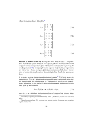
![3. By writing down a general 3 × 3 anti-symmetric matrix (AT = −A), you
should see that it is parametrised by three unknowns (real numbers): A =
A(α, β, γ). In particular, show that any anti-symmetric matrix A can be
written as a linear combination of the {Ej} matrices:
A(α, β, γ) = αE1 + βE2 + γE3, α, β, γ ∈ F. (197)
This says that the set so(3) of 3×3 anti-symmetric matrices is a 3-dimensional
(abstract) vector space with {E1, E2, E3} acting as a set of (abstract) basis
vectors – hence why we denoted them using ‘E’ initially.
4. Using the matrix commutator, [A, B] = AB −BA, as the Lie bracket, prove
that the abstract vector space so(3) is indeed a 3-dimensional Lie algebra
– the special orthogonal algebra. To do this, simply verify that the matrix
commutator [_, _] is a binary operation and that so(3) satisfies the three 3
properties required by a Lie algebra.
Hint: First show that the matrix commutator [_, _] is anti-symmetric and left-
linear in general, then show that it obeys the Jacobi identity in general. It then
suffices90 to show that [_, _] is a binary operation – i.e. that the commutator
[A, B] of any 3 × 3 anti-symmetric matrices A, B is also anti-symmetric, by
showing that (using Einstein summation notation):
[Ei, Ej] = ijkEk
(198)
where ijk is the Levi-Civita symbol defined in tutorial 7.
5. Those of you familiar with vector cross-products will notice the similarity
between the Lie algebra relation: [Ei, Ej] = ijkEk and the cross-product
relation for the standard basis vectors {ej} in 3-dimensions:
ei × ej = ijkek
. (199)
This is because 3-dimensional Euclidean space R3 equipped with the vector-
cross product is indeed a Lie algebra! In-fact, it is identically the same Lie
algebra as so(3) simply presented in another way – we therefore say these
Lie algebras are ‘isomorphic’.
By defining the Lie bracket on R3 to be the cross-product:
[v, u] := v × u, v, u ∈ R3
(200)
90
If the commutator of any basis vectors produces an anti-symmetric matrix, bilinearity then im-
plies that the commutator is a binary operation.
93](https://image.slidesharecdn.com/1f3b3f2a-4e32-4167-891e-7d7de5f1c671-150709175058-lva1-app6892/85/SGC-2014-Mathematical-Sciences-Tutorials-93-320.jpg)
![show that (R3, ×) is indeed a Lie algebra.
Hint: You can essentially copy the proof you used for so(3) or find the
(obvious) isomorphism (one-to-one correspondence) between R3 and so(3)
– which has been hinted at in many ways.
6. In proving that cross-products in R3 form a Lie algebra, we have the bilinear
property in particular. This then shows that the following operator:
[r, _] = r× (201)
is a linear operator, acting on vectors in R3 to give the cross product:
[r, _](v) := [r, v] = r × v. (202)
Recalling the correspondence between linear operators and matrices, it fol-
lows that the operator r× has a matrix representation – this representation is
given by the Lie algebra isomorphism between R3 and so(3):
ej ↔ Ej, u × v ↔ [ui
Ei, vj
Ej]. (203)
In particular, we represent v× by the following matrix (using Einstein sum-
mation91)
v× → [v]× = vj
Ej =
!
0 −v1 v2
v1 0 −v3
−v2 v3 0
(
0
) (204)
(205)
Show explicitly by matrix multiplication, that [v]×u = v × u. Hint: Repre-
sent u as a column vector in the standard basis.
7. Earlier you computed the general odd and even powers, (Ej)2n+1 and (Ej)2n,
of the tangent matrices. If you were observant, you will have realized that:
E4n = E is the same periodic relation that the imaginary unit i4n = i obeys.
This is part of a deeper connection between Lie algebras and Lie groups
given by the ‘exponential map’. For compact connected Lie groups like the
rotation group SO(3), one can recover the entire group from its Lie algebra –
i.e. all information about the rotation group can be obtained from knowledge
of its infinitesimal behaviour about its identity.
91
Recall in 3-dimensions that v = vj
ej = v1
e1 + v2
e2 + v3
e3.
94](https://image.slidesharecdn.com/1f3b3f2a-4e32-4167-891e-7d7de5f1c671-150709175058-lva1-app6892/85/SGC-2014-Mathematical-Sciences-Tutorials-94-320.jpg)
![Formally, we define the matrix exponential of an arbitrary matrix A as:
eA
:=
1
n!
An
, (206)
provided the series converges. Note we define the zeroth power of a square
matrix to be the identity matrix: A0 = I. The matrix exponential obeys the
usual properties of the exponential function except that in general: eAeB =
eA+B, since matrix multiplication does not commute 92.
In general, the exponential map is given by the exponential map of Rieman-
nian geometry – which makes use of the fact that a Lie group is a smooth
manifold. Matrix Lie groups, such the rotation group, SO(3), are just a
special case in which the general exponential map can be expressed as the
matrix exponential.
Q: Show that eθEj is a solution to the matrix differential equation
d
dθ
Rj(θ)|θ=0= Ej. (207)
Hint: Use the series expansion of eθEj and the fact that (θA)n = θnAn for
an scalar θ and any square matrix A.
8. As promised, we now use Lie algebras to establish a fundamental link be-
tween cross-products and rotations. In particular, using the definition of the
matrix exponential, show that the rotation matrices Rj(θ) are given by ex-
ponentiating the tangent matrices which act as a basis for the Lie algebra
so(3):
eθEj
= Rj(θ), (208)
for j = 1, 2, 3.
9. Using previous observations, we can express a rotation about an axis defined
by some unit vector ˆv using our Lie algebra isomorphism and the matrix
exponential. In particular, [ˆv]x = vjEj and:
Rˆv(θ) = eθvjEj
. (209)
This is extremely inefficient, but if you have infinite time, check that the
above expression coincides with that given by ‘Rodrigue’s Rotation For-
mula’. Otherwise, try expanding both expressions to say – first order in
92
The correct relation is given by the Baker-Campbell-Hausdorff formula.
95](https://image.slidesharecdn.com/1f3b3f2a-4e32-4167-891e-7d7de5f1c671-150709175058-lva1-app6892/85/SGC-2014-Mathematical-Sciences-Tutorials-95-320.jpg)
![Exercise 26 By either consulting tutorial 8 or one of your tutors for the axioms of
an abelian group, show that subset of complex numbers with unit length form an
Abelian group.
Hint: Recall that if z, w ∈ C are complex numbers with unit length, then we can
represent them in polar form by: z = eiθ and w = eiφ, where θ and φ are the
principle arguments of z and w, respectively. Therefore, you should parametrize
S1 as the set: {eiθ : θ ∈ R}.
Strictly speaking, we should restrict to θ ∈ [0, 2π) and use modular arithmetic (the
formal term for what you usually do anyway):θ + 2π ≡ θ[mod2π].
Stronger to the previous result, the circle group is in fact a Lie group! To show
this, you could demonstrate that the multiplication map is smooth (simply corre-
sponding to the addition of angles) and that the unit circle S1 is a smooth manifold
(for example, by forming charts from stereographic projections). Since it is com-
pact (closed and bounded) and connected (meaning any two points on the circle are
connected by some path on the circle), it follows that we can reconstruct the circle
group from its Lie algebra via the ‘exponential map’.
Exercise 27 (Circular Reasoning) Wanting to design a bigger, better Orbital Death
Star, the three amigos decide to program a new targeting algorithm with the alge-
bra of Quaternions. However, with the closure of the university (due to Greens riots
regarding their endorsement of environmentally-unsustainable science projects)
and the permanent collapse of the ’BigAir’ server, the three amigos are set on
a quest to find and construct the Quaternion algebra. As such, they decide the cir-
cle group is a good place to start – maybe the rotation group can be reconstructed
as a product of three circle groups?
First take any element z = eiθ of the circle group, then look at its infinitesimal
form by setting the rotation angle θ → δθ, where δθ is infinitesimally small. To
this extent, you can use the first order Taylor series expansion of eiθ to analyze the
structure of S1 about the identity (θ = 0):
z = eßθ
=≈ 1 + iθ. (220)
By replicating the derivation of the Lie algebra for the 3-dimensional rotation
group, show that the lie algebra elements (u(1)) of the circle group are given by:
dz
dθ
= iθ, θ ∈ [0, 2π). (221)
Therefore, we can represent any element of the circle algebra u(1) by iθ – some
angle multiplied by i. Since multiplication of two circle group elements corre-
101](https://image.slidesharecdn.com/1f3b3f2a-4e32-4167-891e-7d7de5f1c671-150709175058-lva1-app6892/85/SGC-2014-Mathematical-Sciences-Tutorials-101-320.jpg)
![sponds to addition of angles (via the properties of the complex exponential), the
Lie bracket on the circle algebra u(1) is given by:
[a, b] = ab − ba. (222)
Show that the elements of u(1) do indeed obey the properties of a Lie algebra with
this Lie bracket.
Hint: Since the multiplication of complex (or real) numbers commutes, this exer-
cise is trivial as [a, b] = 0 ∀a, b ∈ C – i.e. the Lie bracket is zero, hence trivially
satisfies all required properties.
Formally, the circle group is often referred to as the 1-dimensional ‘Unitary group’,
U(1), characterized by the unitary condition:
zz†
= 1 ∀z ∈ U(1), (223)
where † is the ‘conjugate transpose’ – for complex numbers, this is simply the com-
plex conjugate. By the relation eiθ = e−iθ it is clear that all elements of the circle
group satisfy the unitarity condition: eiθeiθ = e0 = 1. As such, the circle group
acts as a building block for all higher-dimensional compact, connected, abelian Lie
groups – that is, all such Lie groups are simply a direct product of circle groups:
Tn = S1 × ... × S1, corresponding to an n-dimensional torus (the 2-dimensional
torus is your familiar doughnut).
Unfortunately, despite being central to the construction of abelian Lie groups, the
circle group does not serve as a building block for quaternions – our desired alge-
braic structure to represent rotations in 3-dimensions. You see this easily by noting
that rotations in 3-dimensions don’t commute (equivalently, the matrix multipli-
cation of rotation matrices isn’t commutative) – hence there is no chance that a
commutative group such as S1 will serve as an appropriate building block.
Finally, as a closing remark on the circle group, one should observe that L2(S1)
– the space of ‘square integrable’ functions95 defined on the unit circle, is simply
the space of periodic functions (we can always normalize the circumference 2π to
any period we want). As such, the representation theory of Lie group S1, gives
rise to Fourier series and Fourier analysis – quintessential to modern mathematics,
engineering, computer science, physics, chemistry, biology and music (acoustic
theory).
95
Lesbegue measurable functions: f ∈ L2
(S1
) =⇒
S1
|f|2
∞.
102](https://image.slidesharecdn.com/1f3b3f2a-4e32-4167-891e-7d7de5f1c671-150709175058-lva1-app6892/85/SGC-2014-Mathematical-Sciences-Tutorials-102-320.jpg)
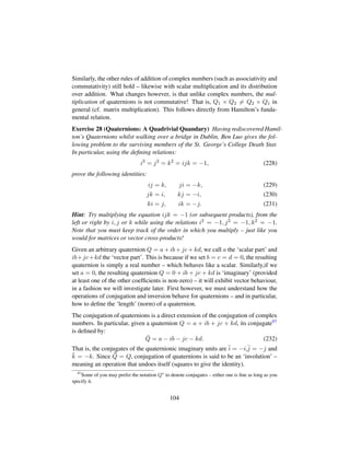
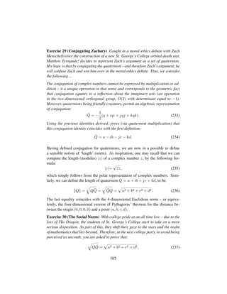
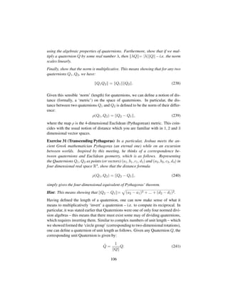
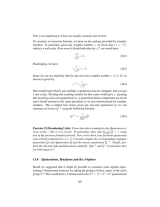
![At the end of the day, it’s neither better to undersell or oversell yourself.
Sure, you want to sell yourself well when applying for jobs, scholarships or
various opportunities – or you may wish to undersell yourself so as not to
alienate oneself from people who are easily intimidated and envious. How-
ever, in your own personal and private inventory of your abilities, one should
strive to be very precise and accurate – this means having a good operational
understanding of your weaknesses and strengths. As a general principle, one
should always be working to improve their weaknesses and capitalize on
their strengths – this alone, will lead to a rise in grades and performance at
university (and life in general).
• Dunning-Kruger effect. “If you’re incompetent, you can’t know you’re in-
competent. [...] the skills you need to produce a right answer are exactly the
skills you need to recognize what a right answer is. –David Dunning.
“Unskilled individuals suffer from illusory superiority, mistakenly rating
their ability much higher than is accurate. This bias is attributed to a metacog-
nitive inability of the unskilled to recognize their ineptitude.[Kruger Dun-
ning, Journal of Personality and Social Psychology, Vol 77(6), Dec 1999,
1121-1134]
“Those persons to whom a skill or set of skills come easily may find them-
selves with weak self-confidence, as they may falsely assume that others
have an equivalent understanding (Impostor syndrome).
In summary, the Dunning-Kruger effect is a rife disease of the mind which
can only be cured with ‘academic maturity’. Since it occurs in the population
at large, it’s not unusual in any respect – for example, recalling Alexander
Pope from 1709:
A little learning is a dangerous thing; drink deep, or taste not the Pierian
spring: there shallow draughts intoxicate the brain, and drinking largely
sobers us again.
Similarly, one can find much earlier statements pertaining to humility and
ability, for example, from Confucius – “Real knowledge is to know the
extent of one’s ignorance.
If you’re going to claim that you’re good or excellent at something (e.g. be-
ing intelligent), take a step back and ask yourself – in what context and by
what measures are these claims met? If someone else claims this, ask your-
self the same thing. On the other hand, if you claim to be bad at something,
take a step outside of yourself and scope out the progress you’ve made – are
114](https://image.slidesharecdn.com/1f3b3f2a-4e32-4167-891e-7d7de5f1c671-150709175058-lva1-app6892/85/SGC-2014-Mathematical-Sciences-Tutorials-114-320.jpg)
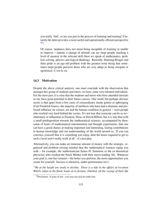
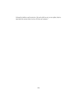
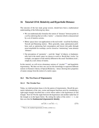
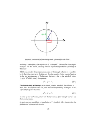
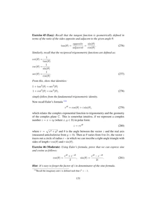
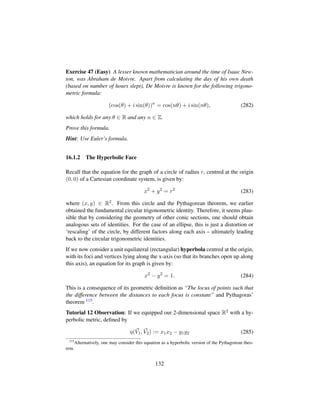
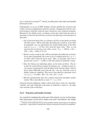
![contraction’ formulas.
Recall that given two vectors v and u in a Euclidean vector space, the Euclidean
‘dot-product’ contains information about their lengths and the ‘angle’ θ between
them:
u ·Euclid v = u v cos(θ). (311)
This special geometric interpretation of the ‘inner product’ (dot-product) is due to
the ‘Cauchy-Schwarz’ inequality, which holds for all positive-definite inner prod-
uct spaces (vector spaces with positive-definite inner-products):
|u · v|≤ u v . (312)
To see this, we simply expand the absolute value (by its definition) and re-arrange
the inequality:
− 1 ≤
u · v
u v
≤ 1. (313)
Now, what monotone function lies between ±1? Cosine of course – in the do-
main [0, π] it is monotone decreasing. Therefore, we can taken the inverse of the
cosine function of both sides of the inequality (reversing it since cosine is decreas-
ing):
0 ≤ arccos(
u · v
u v
) ≤ π, (314)
which allows one to interpret u·v
u v as some geometric angle θ.
Inside a spacetime observer’s light cone, the vector space they generate relative
to their origin is ‘negative definite’ as we partially saw earlier – in particular,
the inner-product of any two future-pointing time-like vectors, U and V , is neg-
ative:
η(U, V ) ≤ 0. (315)
Therefore, inside the light cone, we get the ‘reverse Cauchy-Schwarz inequal-
ity’:
|U ·Lorentz V |≥ V U . (316)
Re-arranging and noting that |U ·Lorentz V |= −U ·Lorentz V for any future-pointing
time-like vectors U, V , we get:
−
U ·Lorentz V
U U
≥ 1. (317)
What trigonometric function satisfies the property that it is always ≥ 1? Hyper-
bolic cosine! Thus, we can define the hyperbolic angle or rapidity between any
145](https://image.slidesharecdn.com/1f3b3f2a-4e32-4167-891e-7d7de5f1c671-150709175058-lva1-app6892/85/SGC-2014-Mathematical-Sciences-Tutorials-145-320.jpg)

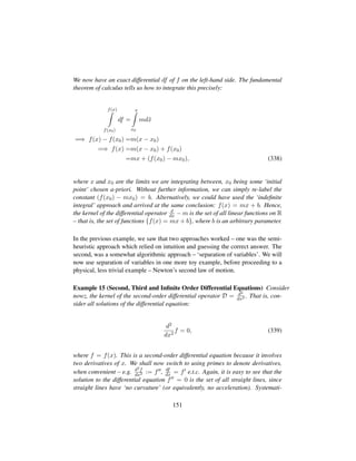
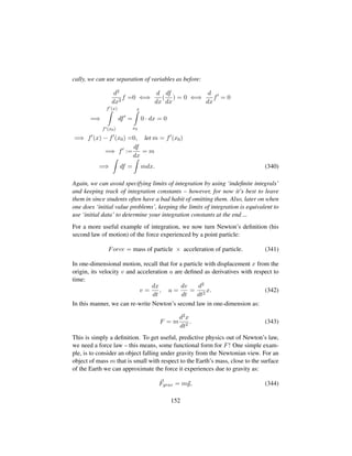
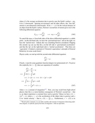
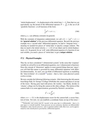
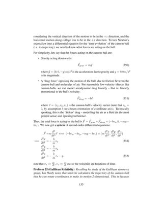
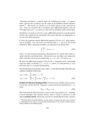
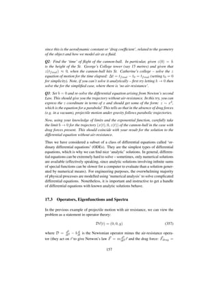
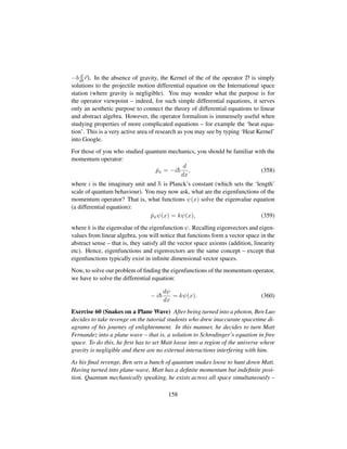
![In general, this is only possible if the function v (y)
g(y) is of a special form – in partic-
ular, if v (y) = λg (y) (for some constant λ), then we can use the identity:
g (y)
g(y)
dy = ln[g(y)] + c, (370)
where c is some constant of integration. This is because we have an exact differen-
tial 139
g (y)
g(y)
dy = d(ln[g(y)]), (371)
allowing us to apply the ‘fundamental theorem of Calculus’.
If the left-hand side, dv(y)
g(y) , is not of this form, either we cannot integrate it or we
must use some special ‘tricks’ to put it into this form.
Problem 27 (A question of separability) Consider the following differential equa-
tion for y as a function of t:
dy
dt
+
5
t
y = t − 2 +
2
t
. (372)
Now try and solve this differential equation for y explicitly in terms of t, using the
method of separation of variables.
Hint: If you can’t complete this problem in 5−10 minutes, move to the next section.
18.2 Integration Factors
For now, we shall consider ordinary first-order differential equations. The integrat-
ing factor method can be used recursively for higher-order differential equations
... if you are lucky. For example, recall the projectile motion problems in tuto-
rial 15 – these were second order differential equations, but effectively amounted
two sequential first order differential equations for the projectile trajectory (first we
solved for velocity, then displacement).
In general, the integrating factor method is useful for solving ODEs of the follow-
ing form:
dy
dx
+ P(x)y = Q(x), (373)
139
Recall that for a function f of one variable – say y, its ‘exterior derivative’ or exact differential
is given by: df = df
dy
dy. The term dy is a differential 1-form – an object which is ‘dual’ to unit
vector ey in the y-direction.
162](https://image.slidesharecdn.com/1f3b3f2a-4e32-4167-891e-7d7de5f1c671-150709175058-lva1-app6892/85/SGC-2014-Mathematical-Sciences-Tutorials-162-320.jpg)
![where P and Q are functions of the independent variable, x. To put this differential
equation into ‘separable form’ (defined earlier), we may consider multiplying it by
some function I(x) to get an exact-differential on both sides.
Assuming this is possible, we have:
I(x)(
dy
dx
+ P(x)y) = I(x)Q(x), (374)
where (dy
dx + P(x)y) is a total derivative. Alternatively, multiplying by dx on both
sides, we get
I(x)(dy + P(x)ydx) = I(x)Q(x)dx, (375)
where I(x)(dy+P(x)ydx) is an exact differential.140 Hence, we must have:
I(x)(
dy
dx
+ P(x)y) =I(x)
dy
dx
+ y
dI
dx
⇐⇒ I(x)(dy + P(x)ydx) =d(I(x)y)
= ydI(x) + Idy
= y
dI
dx
dx + Idy. (376)
Comparing coefficients of dx and dy (linearly independent dual vectors) on the
left- and right-hand sides, we must have:
dI
dx
= I(x)P(x), I(x) = I(x). (377)
Hence we have a separable first-order differential equation for the integrating fac-
tor, I(x):
dI
dx
=I(x)P(x)
=⇒
dI
I
=P(x)dx
=⇒
dI
I
= P(x)dx
=⇒ ln[I(x)] =C + P(x)dx
=⇒ I(x) =e P(x)dx
, set C=0 . (378)
140
Recall that an exact differential, or ‘exterior derivative’ of a function f(x, y) of two variables is
given given by: df = df
dx
dx + df
dx
dy.
163](https://image.slidesharecdn.com/1f3b3f2a-4e32-4167-891e-7d7de5f1c671-150709175058-lva1-app6892/85/SGC-2014-Mathematical-Sciences-Tutorials-163-320.jpg)
![Problem 28 (Party Patrol) In a twist of events, during a “Filius Fogg themed
college party, Alice becomes a bit too rowdy. The Sherrif on duty – Matthew Goss,
decides that it’s time to Taser Alice with the official RA Taser. When dry, the human
skin has a resistance of about 100, 000 Ohms.
To model this tasering process, we can consider Alice to be a resistor of 100, 000Ω
(Ohms) and Matt’s taser to be a discharging capacitor, with a capacitance of C =
100µF (micro farads). This makes the system an ‘RC Circuit’. Using Ohms Law,
we have
V = IR, (384)
between any two points on the circuit, where the voltage V and current I are
functions of time and the resitance R between the two points is constant. Since
capacitance C is related to the voltage and charge Q stored in the taser we have:
Q = CV. (385)
Finally, since current is defined as the ‘rate of flow of charge’ through any chosen
point in the circuit, we have I = dQ
dt . Thus, differentiating the capacitance equation
with respect to t (noting that the capacitance C is constant), we get:
dQ
dt
= I = C
dV
dt
. (386)
Combining this with Ohm’s law and conservation of charge (Kirchoff’s current
law), we get the following differential equation for the voltage V :
dV
dt
+
1
RC
V = 0. (387)
Q0[Easy]: Reproduce the intermediate steps required to derive the above differen-
tial equation. Now, if you like – instead of eliminating the current I, try eliminating
the voltage V and arrive at differential equation for the current I as a function of
time t.
Q1: Is this differential equation separable? If so, re-arrange it to the canonical
form defined at the start of the tutorial.
Q2: Solve this differential equation for the voltage V as a function of time t, where
t = 0 is the time of initial discharge (tasering). To get a unique solution, set the
initial voltage V0 := V (0) to be 150, 000 volts.
Hint: Your solution involve some sort of ‘exponential decay’. Can you think of why
this makes sense physically?
165](https://image.slidesharecdn.com/1f3b3f2a-4e32-4167-891e-7d7de5f1c671-150709175058-lva1-app6892/85/SGC-2014-Mathematical-Sciences-Tutorials-165-320.jpg)
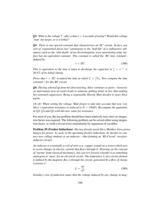
![netic flux through the circuit is given by:
V =
dφ
dt
=⇒ V = L
dI
dt
. (390)
Combing this with Ohm’s Law: V = IR and the conservation of (electrical poten-
tial) energy (Kirchoff’s Voltage law), we get the following differential equation for
the current I flowing through the circuit, as function of time t:
Vin = IR + L
dI
dt
. (391)
Here Vin is the ‘input voltage’, which is constant in time.
Q0[Easy]: If you study physics or engineering, derive the above differential equa-
tion based on the principles outlined. Hint: All the hard work has already been
done.
Q1: Rearrange this differntiale equation into standard form, then solve directly
using ’separation of variables’ find an ‘integration factor’ and then solve it.
Q2: The voltage VR across the resistive element of this circuit (the college fresher),
is given by conservation of energy:
VR = Vin − VL, (392)
where VL is the voltage through the inductor.
Combining this with the above differential equation and using a ‘step-voltage’ in-
put (meaning Vin(t) = 0 for t 0 and Vin = V0 for t ≥ 0), one should get:
VL(t) = V0e−R
L
t
, VR = V0(1 − e−R
L
t
). (393)
Similar to the RC circuit, we can define a special constant – the ‘time constant’
for RL circuit.
In particular, we define the time constant τ for an RL circuit to be the time it takes
for the voltage to drop across the inductor L, to a factor of 1
e of its initial value.
Equivalently, this the time taken for the voltage to rise to within 1
e of its final value
across the resistor (fresher) R.
Using this information, prove that time constant is given by:
τ =
L
R
. (394)
167](https://image.slidesharecdn.com/1f3b3f2a-4e32-4167-891e-7d7de5f1c671-150709175058-lva1-app6892/85/SGC-2014-Mathematical-Sciences-Tutorials-167-320.jpg)
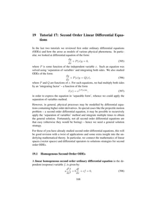
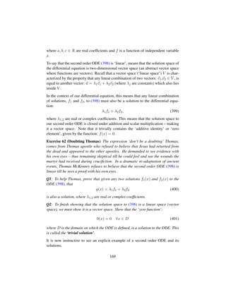
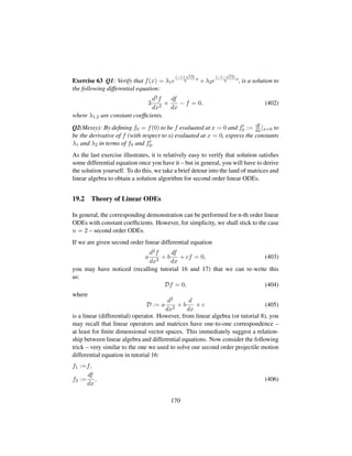
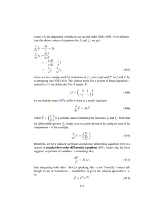
![Here C = is a 2-dimensional vector of constants – CT = [c1c2] is its transpose,
turning it into a row vector (a 1-by-2 matrix). The quantity eMt is the ‘matrix
exponential’ of the matrix Mt (M multiplied by t) – it is well-defined provided
M has a finite operator norm. For now, you don’t have to worry about what this
means – we encountered this object earlier in tutorial 8, where we used Taylor
series to express the exponential of a matrix. Here it suffices to note that we can
compute the exponential of a matrix easily by diagonalizing it – that is, by finding
its eigenvalues (spectrum) and its eigenvectors.
If M is of a ‘nice form’, it will have two linearly independent eigenvectors cor-
responding to two (possibly distinct) eigenvalues. In the case where there is only
one distinct eigenvector, we have to put M into its ‘Jordan normal form’ which
is not too difficult, but well-beyond the technicality we we want to delve into 141.
Nonetheless, assuming we can diagonalize M, then there exists some matrix U
consisting of the eigenvectors of M as its columns, such that:
M = UΛU†
, (413)
where † denotes the conjugate transpose of X (if X is real-valued matrix, this is
just the transpose). The matrix Λ is the 2-by-2 diagonal matrix:
Λ =
¢
λ1 0
0 λ2
(414)
consisting of the eigenvalues λ1,2 of M. Hence, the matrix exponential eMt is
given by:
eMt
= X
¢
eλ1t 0
0 eλ2t
X†
. (415)
In the case the eigenvalues are distinct (non-equal), one will find that the general
solution to our second order linear differential equation (403), is given by:
f(x) = c1eλ1x
+ c2eλ2x
, (416)
where λj are the eigenvalues of the matrix M and cj are constants determined
by ‘boundary values’ (f and its derivative at x = 0) or ’initial conditions’ (if the
independent variable x represents ’time’). Note, we can consider the functions eλ1x
and eλ2x to be ‘basis vectors’ for the 2-dimensional solution space of our ODE –
hence any general vector in that space (i.e. any solution) is necessarily some linear
combination of eλ1x and eλ2x!
141
Alternatively, one can make use of the ‘Putzer algorithm’ to compute the matrix exponential. In
some cases, it is easy to compute directly via Taylor series and brute force – with some intuition.
172](https://image.slidesharecdn.com/1f3b3f2a-4e32-4167-891e-7d7de5f1c671-150709175058-lva1-app6892/85/SGC-2014-Mathematical-Sciences-Tutorials-172-320.jpg)
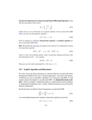
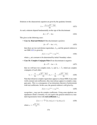
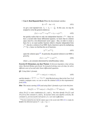
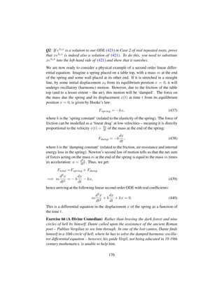
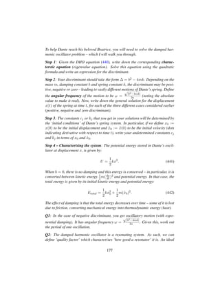
![oscillator would lose no energy per cycle of oscillation. We defined the quality
factor, in the case of negative discriminant, as:
Q = 2π
Energy Stored
Energy Lost Per Cycle
. (443)
Defining the ‘damping ratio’ ξ = b
2
?mk
, find an expression for the quality factor
Q of Dante’s spring in terms of ξ.
Step 5 [SAVE DANTE]: Having determined the solution to a damped harmonic
oscillator, Dante decides to call upon the help of Odysseus (In Latin, Ulysses)
and Aeneas to help him design a ‘spring catapult’. This will eject Dante from the
10th circle into Paradise, where he can be reunited with his lost love, Beatrice.
Assuming Dante weighs m = 70kg and that Paradise is 1000km in the vertical
direction from hell’s 10th circle, workout some possible set of values for the spring
constant k, damping coefficient b as well as initial displacement x0 and initial
velocity 9x0 which will allow Dante to reach Paradise.
To do this, assume that Dante is ejected from the Spring catapult when it reaches
its maximum displacement (limited by the stretchiness of the string) – at this in-
stant, Dante will leave the spring with an upward force of md2x
dt2 and some velocity
dx
dt . Assuming that the force of gravity acts downward on him once he leaves the
spring: F = −mg (g = 10m/s2), Dante will need sufficient exit velocity to reach
paradise.
Hint: Oscillatory motion (negative discriminant) occurs when the motion is under-
damped. In this case the spring oscillates about its equilibrium position, with an
exponential envelope damping the motion so after sufficient (infinite) time the os-
cillations cease – the spring then remains at equilibrium. Over-damped motion
occurs when the discriminant is positive and will typically lead to the spring re-
turning to equilibrium without oscillation.
Hint: This problem is not really well-defined and so might not be (easily) solvable.
So you can re-interpret it to give something sensible and solvable.
The last exercise should illustrate that even for a deceptively ‘simple’ system as
the damped harmonic oscillator, there are a lot of fine details regarding the time-
evolution and behaviour of the system. Such behaviour intricately depends on the
constants that appear in the second order ODE governing its motion.
To finish, we shall look at a more explicit demonstration of second order ODEs.
In particular, we will look at the LRC circuit. In particular, recall from tutorial
16 the examples of an RC and LR circuit. These circuits involved a resistive
178](https://image.slidesharecdn.com/1f3b3f2a-4e32-4167-891e-7d7de5f1c671-150709175058-lva1-app6892/85/SGC-2014-Mathematical-Sciences-Tutorials-178-320.jpg)
![element R, a capacitor (charged storage device) C and some inductor (coil of wire)
L. What happens when you shove all three elements together in a series circuit?
To answer this question, you may use Kirchoff’s Laws (conservation of energy
and charge) along with the defining expressions for inductance (Faraday’s law),
resistance (Ohm’s law) and Capacitance to obtain a dynamical equation for the
time evolution of the LRC circuit.
Exercise 67 The current I(t) (time rate of flow of charge: I = dq
dt ) flowing through
any element of a series LRC circuit at time t, is governed by the following second
order linear ODE:
[
d2
dt2
+
R
L
d
dt
+
1
LC
]I(t) = 0, (444)
where R is the resistance, L is the inductance and C is the capacitance.
Q0: If you who have studied circuits, derive the above differential equation.
Q1: The LRC circuit is simply a ‘re-hash’ of the damped harmonic oscillator.
Looking at the coefficient of dI
dt we see that the equivalent ‘damping constant’ is
given by R
L – correctly suggesting that the resistor acts to ‘oppose’ the flow of
charge (current). Further more, if we multiply through by L, coefficient 1
C of I(t)
suggests treating the capacitor as some ‘spring constant’ type term. This makes
sense in that a capacitor ‘stores energy’ (charge) in the manner that a spring stores
potential energy.
Solve the differential equation for the three different cases, depending on the sign
of the discriminant:
∆ =
(R
L ) − 4
LC
2
. (445)
Now pick some values of I(0), 9I(0), R, L and C and determine a unique solution
– this should correspond to only one case. Graph the current I(t) as function of
time t for the solution you get.
Q2: Define ω0 = 1?LC
, to be the ‘natural frequency’ of our LRC system. This is
the frequency our system would oscillate at without ‘damping’ (without resistance)
– i.e. a perfect resonator. Now define ‘nerper frequency’ α to be:
α =
R
2L
. (446)
Re-write the LRC differential equation in terms of ω0 and α.
Q3: The ‘damping ratio’ ξ for an LRC circuit characterises the ‘energy loss’ with
179](https://image.slidesharecdn.com/1f3b3f2a-4e32-4167-891e-7d7de5f1c671-150709175058-lva1-app6892/85/SGC-2014-Mathematical-Sciences-Tutorials-179-320.jpg)
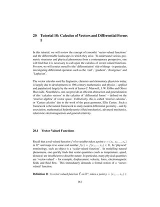
![Rn and maps it to a vector F(x) ∈ Rn. Mathematically 143,
F : Rn
→ Rn
p →F(p). (448)
We can represent a vector-valued function several ways. First, given some basis
{ej} for Rn, we can represent a vector-valued function simply by its component
functions Fj:
F(x) = (F1(x), F2(x), ..., Fn(x)) = (F1(x1, ..., xn), ..., Fn(x1, ..., xn)). (449)
Note that each component function, Fj(x1, ..., xn) is a function of n variables.
More explicitly, we can represent a vector-valued function in a geometrically in-
variant form:
F(x) = F1
(x)e1 + F2
(x)e2 + ... + Fn
(x)en (450)
expanding it in terms of the standard basis vectors ej multiplied by the component
functions Fj(x). [Recall the convention of ‘raising’ the indices of the component
functions and lowering those of the standard basis vectors – the Einstein summation
convention explained in tutorial 7].
Example 16 In physics, ‘force’ is formally a vector quantity. For example, given a
particle of mass m, the force it experiences depends on the nature of its trajectory
through space, via Newton’s second law:
F = ma. (451)
If we let x = (x1, ..., xn) be the displacement vector of the particle, then Newton’s
second law tells us that the force F is a vector-valued function of the displacement
x as follows:
F(x) = m
d2x
dt2
= m(:x1, :x2, ..., :xn). (452)
Problem 30 (The Garden of Forking Paths) Caught in a surreal twist of George
Louis Borges’ ‘garden of forking paths’, a student of the mathematical sciences
finds themselves in the middle of a garden. To their left and their right, lay two
opposing paths – forking off into darkness. The student is forewarned, that upon
143
Strictly speaking, F maps it to the ‘tangent space’ Tp(Rn
) at p (the space of all tangent vectors
at p). However, due to affine parallelism, this is canonically isomorphic to the vector space Rn
– so
we can ignore the distinction.
182](https://image.slidesharecdn.com/1f3b3f2a-4e32-4167-891e-7d7de5f1c671-150709175058-lva1-app6892/85/SGC-2014-Mathematical-Sciences-Tutorials-182-320.jpg)
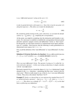
![Since the coordinates x1, x2, x3 are all independent, it follows that:
∂xj
∂xk
= δj
k, (469)
whence the collection {dxj} satisfies the defining property of a dual basis.
Exercise 69 (Voices in the wind) After meeting Satyr and viewing their future self,
our student is now confronted by a gale – carrying with it, voices from their past
life. Amidst this chaotic cacophany, the student hears scattered teachings of di-
mensional analysis.
Q1: To banish the gale, the student must work out the relationship between the
dimensions of the basis vectors ej = ∂j and the dual vectors θj = dxj. Do this.
Hint: To compute the dimensional relation required, you can use the definition of
a dual basis: θj(ej) = δj
k and note that the Kronecker delta is a dimensionless
quantity.
Q2: You are now told that the differential 1-forms (dual vectors) dxj represent
‘infinitesimal length elements’. For this to make sense, it follows that [dxj] = L,
where L is some unit of length. From this and your result in Q1, compute the
dimensions of the tangent vector (partial derivative operator) ej = ∂j.
The name differential ‘1-form’ is suggestive of the fact that there exists, in general,
‘differential k-forms’, where k is some non-negative integer. Such a suggestion is
true – where k has an upper limit of k = n, n being the dimension of your vector
space (for us, n = 3). The reason for this limit will become apparently shortly. For
now, it necessary it introduce a special ‘product’ between differential forms – the
‘exterior product’. Under this product, differential forms form an ‘algebra’ known
as the ‘exterior algebra’. As it turns out, any finite dimensional vector space (e.g.
R3) automatically comes equipped with an exterior algebra.
Definition 14 (Exterior Product) Given two differential 1-forms, ω and θ, their
exterior product ∧ is defined as:
ω ∧ θ, (470)
which is a differential 2-form. Furthermore, ∧ is characterised by the following
properties:
1. Antisymmetry:
ω ∧ θ = −θ ∧ ω. (471)
2. Bilinearity:
(λ1ω + λ2φ) ∧ θ = λ1ω ∧ θ + λ2ω ∧ φ, (472)
188](https://image.slidesharecdn.com/1f3b3f2a-4e32-4167-891e-7d7de5f1c671-150709175058-lva1-app6892/85/SGC-2014-Mathematical-Sciences-Tutorials-188-320.jpg)
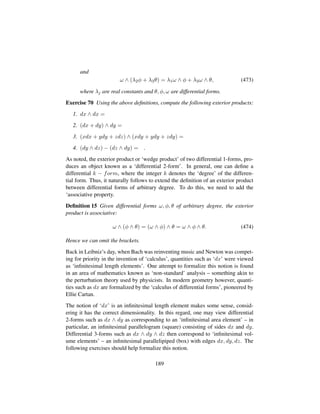
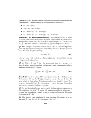
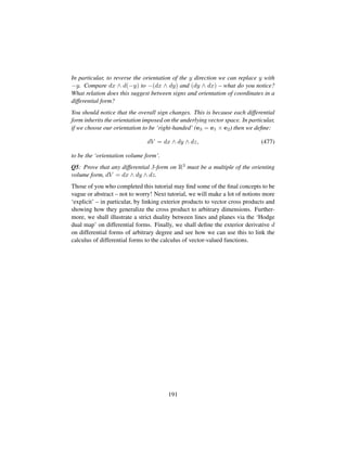
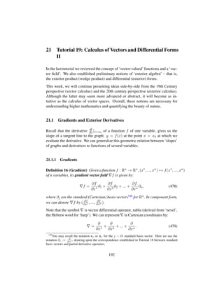
![Hence, from this perspective, the gradient f is simply given as the above oper-
ator acting on f. Furthermore, is a linear differential operator (since it can be
represented as as sum of linear differential operators) – hence it obeys the Leibniz
product rule:
(fg) = f g + g f, (480)
and linearity property:
(c1f + c2g) = c1 f + c2 g, (481)
for arbitrary differentiable functions f, g.
To get an intuition of how the ‘gradient vector field’ behaves, we first illustrate its
first fundamental property – the gradient of a function is a vector field which points
in the direction of the maximum (positive) rate of change of the function and whose
magnitude is equal to the ‘slope’ of the graph of the function in that direction.
Example 18 (A Sunburnt Country) Nostalgic over happier times, Dr. Claire Wadding-
ton decides to read a poem by Dorothea Mackellar while partying in a desert music
festival with Angus Turner: “I love a sunburnt country, A land of sweeping plains,
Of ragged mountain ranges, Of droughts and flooding rains.... Realizing that she
is surrounded entirely by barren sweeping plains, she recalls her time in Northern
England. To this extent, she decides that she can approximate the hills between
Durham and Edinburgh by Circular or Elliptical Paraboloids.
If we define a function f(x, y) = h−(x2+y2) of two-variables, then the graph of a
circular paraboloid in 3-dimensions, is given by: z = f(x, y). Letting z represent
the altitude of a point on the hill (whose peak height is h), and (x, y) represent
coordinates on 2-dimensional map (restricted so that x2 + y2 ≤ h), we can draw
the ‘level sets’ of f or ‘contour lines’ of the hill by drawing the concentric circles,
z = f(x, y) for different values of z [Do this as an exercise].
The gradient vector field of f, is given by:
f =
∂f
∂x
∂x +
∂f
∂y
∂y = −2x∂x − 2y∂y. (482)
This points in direction (x, y), which is the direction opposite the radius vector
r = x∂x + y∂y – as such, it is orthogonal to the level sets (circles) of f. Note that
z = 0 corresponds to the summit of the hill – which is where the gradient vector
field points towards (increasing altitude). Since the gradient field is perpendicular
to the contour lines, it points in the direction of the maximum rate of increase of
z = f(x, y) – i.e. the steepest ascent up the hill.
193](https://image.slidesharecdn.com/1f3b3f2a-4e32-4167-891e-7d7de5f1c671-150709175058-lva1-app6892/85/SGC-2014-Mathematical-Sciences-Tutorials-193-320.jpg)
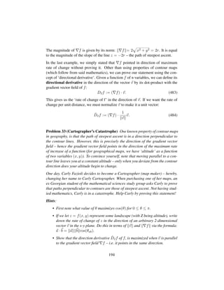
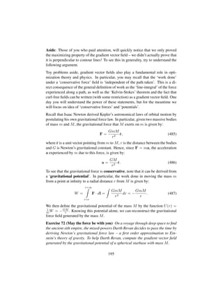
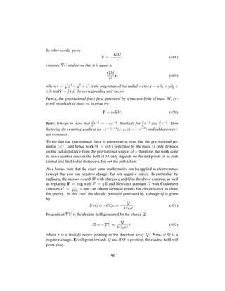
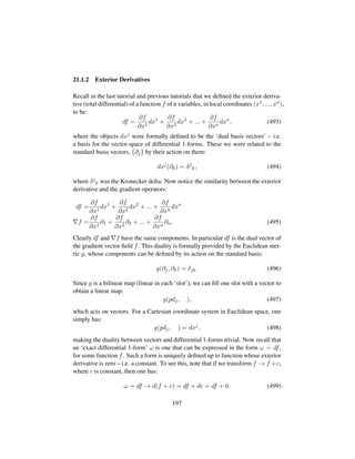
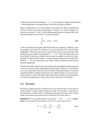
 = lim
V →p
S=∂V
1
V
F · dS. (502)
Note that the quantity
S=∂V
is the surface integral over the boundary surface
of V and dS = ndS is the outward-pointing normal vector of (perpendicular
to) S, whose magnitude dS is the infinitesimal surface area at any point on S.
Furthermore, note that this definition of divergence does not depend on the explicit
surface chosen – if it did, it would be useless!
As such, the divergence measures the ‘source’ or ‘sink’ behaviour of a vector field
at any point. To see this explicitly, consider the following example.
Example 19 (Fracking Well) Fracking is a process by which water can be pumped
deep below the Earth into fine rock formations to build pressure, crack rocks and
release natural gas for extraction. At the top of some well site, the diffusion of
the natural gas can be modelled by a vector field F = x∂x + y∂y + 100z∂z – i.e.
a somewhat upward ‘conical flow’. The units of the components is flow rate of
natural gas per second per unit area – i.e. [Mass]
[Time][Area] The divergence of this vector
199](https://image.slidesharecdn.com/1f3b3f2a-4e32-4167-891e-7d7de5f1c671-150709175058-lva1-app6892/85/SGC-2014-Mathematical-Sciences-Tutorials-199-320.jpg)
![field is given by:
Div[F] = · F
=
∂Fx
∂x
+
∂Fy
∂y
+
∂Fz
∂z
=1 + 1 + 100
=102, (503)
ignoring units. Since this divergence is positive, the well opening can be viewed
mathematically as a ‘source’ for the natural gas vector field. You can plot this
vector field to see that it does indeed ‘look’ like a source.
If one were to consider another operation – for example, Carbon sequestration,
then you may write a carbon vector field as: F = −x∂x − y∂y − 10z∂z at the
top of some pump leading underground, for example. Computing the divergence
should give you a negative quantity – hence corresponding to the top of the pump
being a Carbon sink.
Example 20 (Electric Charge) Due to Michael Faraday, we often do calculations
in electromagnetism with an artificial quantity – the ‘electric field’ E defined in
terms of the force experienced by a positive test charge due to another given charge
configuration. In particular, an electric charge Q generates an electric field defined
by E = 1
QF, where F is the force experienced (a measurable quantity) by a positive
test charge in field of Q.
Regardless of the nature of the charge Q, at far enough distances, we can approx-
imate the electric field generated by Q as that of a point charge via Coulomb’s
law:
E =
Q
4π 0r2
ˆr, (504)
where r = x
r ∂x + y
r ∂y + z
r ∂z is a unit vector pointing outward from Q (placing Q
at the origin (0, 0, 0)).
Without a second thought, Kate Lindley is told that ‘positive charges’ act ‘sources’
for electric field lines and negative charges act as ‘sinks’. Graphically, this makes
sense if we plot E. However, if we try to formalize this notion, one might think that
in the neighbourhood of positive charges an electric field has positive divergence
– and around negative charges its divergence is negative. Is this really the case?
Considering a point-charge at the origin (0, 0, 0) and computing its divergence, we
200](https://image.slidesharecdn.com/1f3b3f2a-4e32-4167-891e-7d7de5f1c671-150709175058-lva1-app6892/85/SGC-2014-Mathematical-Sciences-Tutorials-200-320.jpg)
![get:
Div[E] = · E
=
∂Ex
∂x
+
∂Ey
∂y
+
∂Ez
∂z
=(
1
r3
−
3(x)
r4
xr−1
) + (...) + (...)
=
3
r3
−
3(x2 + y2 + z2)
r5
=0, (505)
since Ex = Q
4π 0r2
x
r = Q
4π 0
xr3, e.t.c. Oh no! What is going wrong here? The
real problem is that electric field E in its given form is not ‘defined’ at the origin
– technically speaking, this a hole in the solution space to Maxwell’s equations for
electromagnetism.
If we use Gauss’ law to compute the charge enclosed by a sphere around the origin,
then we must take into account that a point charge at the origin has an infinite
charge density at the origin and has zero charge density everywhere else. To take
this into account, we need the 3-dimensional Dirac delta distribution δ3(r) – which
is (informally speaking) defined to be infinity at r = 0 and zero everywhere else.
In this manner, we can write:
· E =
ρ
0
= 4πQδ3
(r). (506)
Since V δ3(r)dV = 1 (the volume integral for a volume V enclosing the origin –
by properties of the Dirac Delta), we recover Q as the charge by Gauss’ law.
Note that the concepts in the last example apply directly to Newtonian gravity, by
consideration of the gravitational field and Gauss law applied to gravity. A more
satisfying explanation for this phenomena is found readily in ‘De Rham Coho-
mology’, relating the concept of ‘closed differential forms’ and ‘non-exact differ-
ential forms’ to topology and a generalized notion of ‘charges’ and conservation
laws.
Problem 34 In fluid mechanics, a fluid is classified as ‘incompressible’ if the di-
vergence of its velocity vector field is zero:
Div[F] = 0. (507)
Similarly, a fluid can be called ‘vortex-free’ if its ‘curl’ is zero (another vector dif-
ferential operator). Fluids with vortices have non-zero circulation at various points
201](https://image.slidesharecdn.com/1f3b3f2a-4e32-4167-891e-7d7de5f1c671-150709175058-lva1-app6892/85/SGC-2014-Mathematical-Sciences-Tutorials-201-320.jpg)
![– i.e. the line integral of the velocity vector field about a closed loop containing
a vortex is non-zero. Loosely speaking, if you integrate around two vortices of
equal magnitude rotating in the opposite direction, the circulation is zero – hence
establishing the beginnings of a notion of duality between vortices and conserved
charges from electromagnetism.
Ignoring these concepts for now, consider a fluid with a single counter-clockwise
vortex modelled by the velocity vector field:
v = −y∂x + ∂y. (508)
Such a vector field arises as the curl of the vector field: 1
2
—
x2 + y2 + z2∂z. One
result of vector calculus is that the divergence of a vector field arising as the curl
of another vector field, is zero. Hence a true vortex has zero divergence – in some
regime (linear perhaps), they are conserved quantities.
Q1:Show that for v = −y∂x + ∂y, one does indeed have Div[v] = 0.
Q2: Given an arbitrary vector field F = Fx∂x + Fy∂y + Fz∂z expressed in a
Cartesian coordinate basis, its curl is a vector field defined by the expression:
× F =
¢
∂Fz
∂y
−
∂Fy
∂z
∂x +
¢
∂Fx
∂z
−
∂Fz
∂x
∂y +
¢
∂Fy
∂x
−
∂Fx
∂y
∂z.
Using this expression as well as the definition of the divergence, prove that Div[ ×
F] = ·( ×F) = 0. This establishes our previous statements in some generality.
Hint: You will need to Clairaut’s theorem – that is, partial derivatives of a (‘ap-
propriately defined’) function commute.
21.3 Hodge Dual, Closed and Exact Forms
For next time ... perhaps.
202](https://image.slidesharecdn.com/1f3b3f2a-4e32-4167-891e-7d7de5f1c671-150709175058-lva1-app6892/85/SGC-2014-Mathematical-Sciences-Tutorials-202-320.jpg)
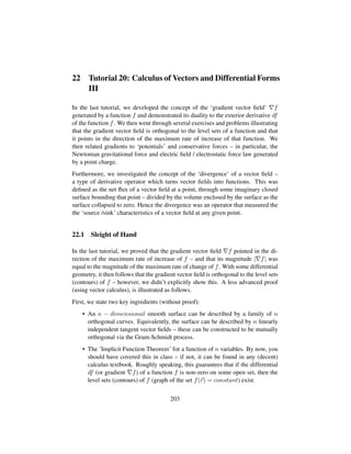
![Proof 2 (Orthogonality of Gradient and level sets) Given a function f on n vari-
ables, (x1, ..., xn) ∈ Rn, one defines a ‘level set’ of f (generalization of the notion
of ‘level curves’ to ‘level hypersurfaces’) as the set of points such that:
f(x1
, ..., xn
) = c, (509)
for some chosen constant c. Therefore, the family of level of sets of f is a parameter
family generated by c (as c varies) – the union of this family is thus the ‘contour
graph’ or ‘level graph’ of f. If the gradient f of f (or exterior derivative df)
is non-zero at some point y = (y1, ..., yn) (with f(y) = c), then the implicit
function theorem implies that the pre-image of C is a submanfiold of Rn – i.e.
the set {x ∈ Rn : f(x) = c} is a smooth hypersurface in Rn. This means it
is generated by n − 1 independent curves, with well-defined tangent vector fields
(velocity vectors) to each curve.
With the existence of a level set established, we parametrized one of the n−1 curves
in the level set by the vector function rc(t) = (x1(t), ..., xn(t)), where c labels the
level set (contour) and t is our parameter. Evaluating our original function f on
this curve and taking its exterior derivative t, we find
df =
∂f
∂t
dt
=[
∂f
∂x1
dx1
dt
+ ...
∂f
∂xn
dxn
dt
]dt. (510)
However, we know that f(rc(t)) = c (by construction of the level set), hence it
follows that: df
dt |rc(t) = 0. Hence, we have:
[
∂f
∂x1
dx1
dt
+ ...
∂f
∂xn
dxn
dt
] = 0. (511)
Now notice that the quantity on the left-hand side of this equation is simply the dot
product of the two following vectors:
f =
∂f
∂x1
∂1 + ... +
∂f
∂xn
∂n
9rc =
dx1
dt
∂1 + ... +
dxn
dt
∂n, (512)
evaluated along the curve given by rc(t) in a level set of f labelled by c. The vector
f is the gradient of f and 9rc is the tangent (velocity) vector to the curve rc(t).
Since · 9rc = 0 as shown above, it follows that the gradient is orthogonal to the
curve rc(t). Repeating this argument for all other curves generating the level set
204](https://image.slidesharecdn.com/1f3b3f2a-4e32-4167-891e-7d7de5f1c671-150709175058-lva1-app6892/85/SGC-2014-Mathematical-Sciences-Tutorials-204-320.jpg)
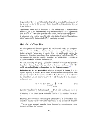
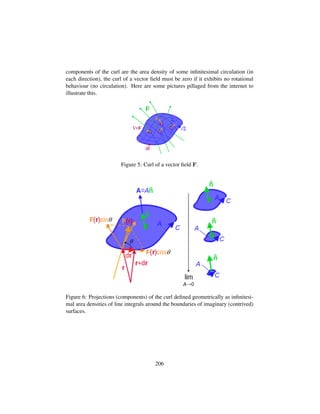
![To get a clearer idea, we shall now give an algebraic definition of the curl as well
some examples and problems. Given a vector field148 F = F1∂1 + F2∂2 + F3∂3,
expressed in the Cartesian basis {∂1, ∂2, ∂3} = {∂x, ∂y, ∂z} for R3, its curl is given
by the following formula:
( × F) = ijk
(∂iFj)∂k
= ijk
(
∂Fj
∂xi
)∂k
=(
∂F3
∂y
−
∂F2
∂z
)∂x − (
∂F1
∂x
−
∂F3
∂z
)∂y + (
∂F2
∂x
−
∂F1
∂y
)∂z. (514)
Note that in the first line, we used the Einstein summation convention as well as the
‘Levi-Civita’ or ‘Permutation’ symbol – defined in earlier tutorials. These give an
elegant way to remember the curl. Alternatively, to remember the explicit formula
in the last line, you can think of the curl informally as the determinant of a 3-by-3
matrix with a row of the standard basis vectors [∂x∂y∂z] in the first line, the partial
derivative operators [ ∂
∂x
∂
∂y
∂
∂z ] in the second line and a row of the components of F
in the third line: [F1F2F3]. The derivative operators in the second line act on the
components in the third line of the matrix (taking partial derivatives of F), whilst
the basis vectors in the first row multiply everything – this ensures that the result is
a vector field (not a function):
∂x ∂y ∂z
∂
∂x
∂
∂y
∂
∂z
F1 F2 F3
.
We now proceed to some examples and problems.
Example 21 (Curl of a Gradient) In an ideal gymnasium, nobody in their right
mind curls in the squat racks. Similar to the ideal gym squat rack, a gradient vector
field has ZERO CURL. This is an extremely important and fundamental property
of gradient vector fields – one which is responsible for the statement that the ‘work
done to move a particle in a conservative force field, is independent of the path
taken’. In other words, it relates to path independence of line integrals of gradient
vector fields (with some minor technicalities).
To prove this statement, consider a function f of three Cartesian variables (x, y, z).
148
Recall that ∂j := ∂
∂xj is both a differential operator (partial derivative) and the standard basis
vector in the direction of the Cartesian coordinate xj
.
207](https://image.slidesharecdn.com/1f3b3f2a-4e32-4167-891e-7d7de5f1c671-150709175058-lva1-app6892/85/SGC-2014-Mathematical-Sciences-Tutorials-207-320.jpg)
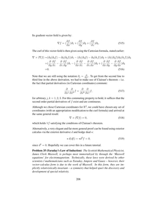
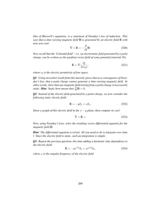
![23 Tutorial 21: Coordinate Systems and Scale Factors
By now, all of you will have come across more than one type of ‘coordinate sys-
tem’. For example, in two dimensions you will have used rectangular (Cartesian)
coordinates, (x, y), as well as ‘polar coordinates’, (r, θ). Depending on the sym-
metries of your problem, each coordinate system would have had its advantages
and disadvantages.
In general, there are an infinite number of coordinate systems you could use to set-
up a problem. However, for spaces such as R2 and R3 equipped with a Euclidean
metric, there is a special (finite) class of coordinate systems known as ‘separable’
coordinate systems. Such a term arises from the fact that the Laplace operator
is separable in these systems – meaning that the Laplace equation is a differen-
tial equation that can be solved by ‘separation of variables’. More generally, the
Hamilton-Jacobi equations are separable in such coordinate systems.
In this tutorial, we will explore a few examples of different 2-dimensional and 3-
dimensional coordinate systems. In particular, we will develop several concepts
and ideas in a ‘geometrical viewpoint’. This should help you gain some physical
intuition behind objects such as the ‘Jacobian determinant’ as well as change-of-
variables.
23.1 Orientation and Measure
Recall that if we are integrating a function f = f(x) of one real variable x ∈ R,
we write:
I =
L
f(x)dx. (525)
The L here denotes the subset of the real line R which we integrate over. For most
integrals, this is just some interval149 L = [a, b]. One way to view the process
of integration is in terms of an operator (a ‘measure’) acting on a function. In
particular, we can view the previous integral I as the operator
L
dx (526)
acting on the function f. This assigns some value to f – it’s measure (Riemann
integral) on the set L (e.g. over an interval L = [a, b]). Such an abstraction,
149
Note that strictly speaking, it doesn’t matter whether or not you include the endpoints – if the
integral exists / converges, then you can take a limit which features the endpoints.
210](https://image.slidesharecdn.com/1f3b3f2a-4e32-4167-891e-7d7de5f1c671-150709175058-lva1-app6892/85/SGC-2014-Mathematical-Sciences-Tutorials-210-320.jpg)
![turns out to be very powerful and useful – for example, the study of probability
measures. Collectively, it is part of a beautiful area of mathematics known as
‘measure theory’.
Fundamental to the construction of a measure
L
dx on the real line R, is the exis-
tence of the object ‘dx’. By now, you should know that this is not just some hazily
defined ‘infinitesimal’ quantity along the x − axis – it is in-fact a well-defined
‘differential 1-form’. Geometrically, not only does it represent an infinitesimal line
element in the x direction, it also represents an ‘orientation’ on the x-axis. This
orientation is in the positive x direction. Technically, we could assign an opposite
orientation by defining dl = −dx in our definition of the measure,
L
dl.
For one-dimensional integrals, the notion of orientation may seem trivial. How-
ever, generalizing to integrals over surfaces, volumes and general n-dimensional
oriented manifolds, there are always two possible choices of ‘orientation’ defined
– this is encoded in an object known as the ‘orienting n-form’.
23.2 Smooth Curves
When we perform an integral f(x)dx, we are integrating the function f along
the x-axis representing the real line R. However, in general, one can integrate
functions along an arbitrary curve. Such integrals form a class known as line inte-
grals.
A curve is a 1-dimensional manifold, meaning it can be parametrised by one vari-
able. In a Euclidean space such as R2 or R3, we can represent this curve by the
functional equations (in the standard Cartesian basis):
γ(t) = x(t)e1 + y(t)e2, t ∈ L (527)
and
γ(t) = x(t)e1 + y(t)e2 + z(t)e3, t ∈ L (528)
where ej are the standard basis vectors in the x, y and z directions and L is some
subset of R – e.g. L = [0, 1] or L = R itself. In this manner, we can view γ(t)
as the position vector for some motion. This means, that for each value of t, we
assign a vector γ(t) which starts at the origin 0 and points to some location on the
curve.150
150
Such a construction is only possible for affine spaces – such Euclidean vector spaces. In general,
one must be more subtle in defining and representing a curve.
211](https://image.slidesharecdn.com/1f3b3f2a-4e32-4167-891e-7d7de5f1c671-150709175058-lva1-app6892/85/SGC-2014-Mathematical-Sciences-Tutorials-211-320.jpg)
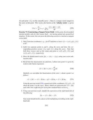
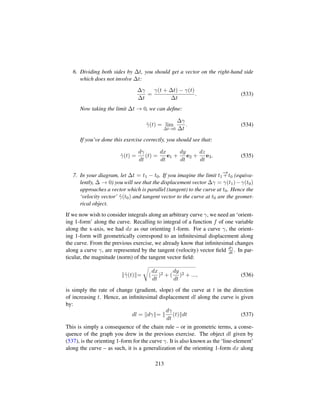
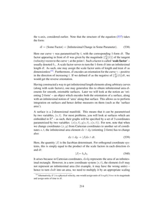
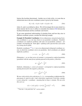
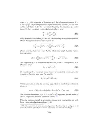
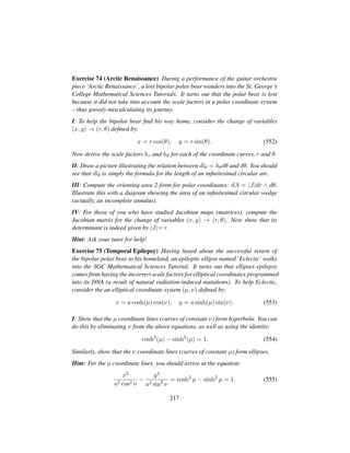
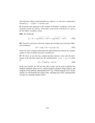
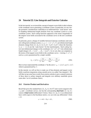
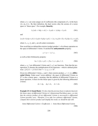
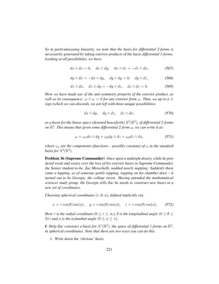
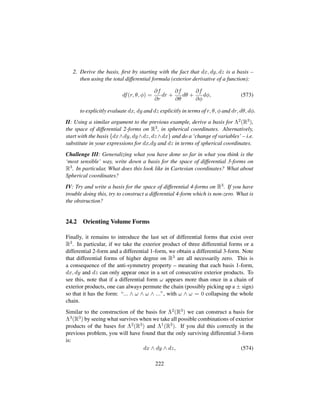
![(up to a ± sign or some permutation of x, y, z). Note that so far, we have always
chosen the cyclic convention: x → y → z → x when ordering our differential 1-
forms – this is intentional as it corresponds to the choice of a ‘right-handed orien-
tation’ on our vector space, R3. Such an orientation is the ‘standard orientation’
for 3-dimensional Euclidean space. In particular, for R3 we have that:
1 = dV = dx ∧ dy ∧ dz, (575)
is the ‘orienting volume 3-form’. By order of the differential 1-forms dx, dy, dz,
it defines an orientation on R3. Furthermore, geometrically, one may think this as
representing an infinitesimal cube (or parallelipiped) with sides of length dx, dy
and dz – giving it dimensions of ‘volume’ (Length3).
In general, for an n-dimensional inner-product space (vector space equipped with
an inner-product or metric tensor) such as Rn, one can equip it with an orienting
volume n-form. This gives the space an orientation, as well as a way to measure
‘volumes’ – the orienting volume appears when performing volume integrals on
the space. It also acts a basis for forms of the highest degree on that space – any
differential n-form must be some scalar multiple of it.
Now that we have established the idea that differential p-forms (where p is some
integer) behave like ‘abstract vectors’ in a linear space (under ‘addition’), we can
explore the relation between exterior products, differential forms and the vector
calculus we already know and love.
Exercise 76 (Choice of Orientation) When questioned about her Orientation dur-
ing ‘true colours’ week, a spherical coordinate system is caught-off guard. Real-
izing that she has lost her orienting volume 3-form, she decides to construct a new
one.
I: If you are (left)right-handed, construct a (left)right-handed orienting volume
form in spherical coordinates. [If you are genuinely ambidextrous, construct two
oppositely oriented coordinate systems with each hand, simultaneously (writing
with two pens at once)]. You can do this by computing dx, dy, dz in terms of
spherical coordinates (r, θ, φ) and the spherical basis 1-forms: (dr, dθ, dφ), then
substituting your results into the expression dV = dx∧dy∧dz (for the right handed
system). Alternatively, for the left-handed system, use dVLefty = −dx ∧ dy ∧ dz.
II: Now, use your results from Tutorial 21 to construct the orienting volume 3-form
via the expression:
dV = hrdr ∧ hθdθ ∧ hφdφ = |J|dr ∧ dθ ∧ dφ. (576)
223](https://image.slidesharecdn.com/1f3b3f2a-4e32-4167-891e-7d7de5f1c671-150709175058-lva1-app6892/85/SGC-2014-Mathematical-Sciences-Tutorials-223-320.jpg)
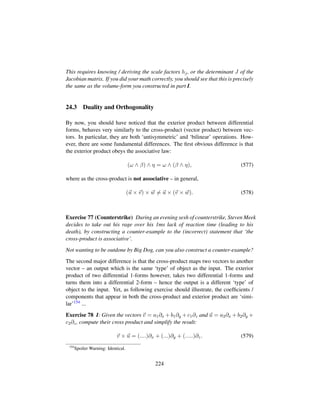
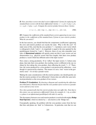
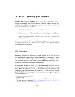
![Hence the configuration space of a physical system naturally takes the form of a
‘tangent bundle’ 162, denoted TM.
Abstraction aside, we now consider the Lagrangian for a simple system (e.g. a
point-particle moving with constant acceleration) with a generalized coordinate q
and a generalized velocity 9q = dq
dt . The Lagrangian L = L(q, 9q) for this system is
a function of q and 9q, defined on the configuration space 163 TM.
The action S[L] corresponding to this Lagrangian L, is given by:
S[L] = L(q, 9q) = L(q, 9q)dt. (606)
We can compute the variation of this action δS[L] by using integration by parts and
computing the variation of the Lagrangian: δL. Note that to compute the variation
of the Lagrangian, δL, we simply use the same rules as we do when computing a
total differential (or ‘exterior derivative’). In particular, we have
δL(q, 9q) =
∂L
∂q
δq +
∂L
∂ 9q
δ 9q (607)
Note that we have assumed that the Lagrangian L does not explicitly depend on
time t. It only depends on t implicitly through q(t) and 9q(t). If it did explicitly
depend on t, e.g. for a system with a time-varying potential energy U(t), then we
would just include an extra term: ∂L
∂t in the variation of L.
Therefore, we have:
δS[L] =δ Ldt
= δLdt
= (
∂L
∂q
δq +
∂L
∂ 9q
δ 9q)dt (608)
Note that the variation ‘operator’ δ commutes with derivative operators. Hence for
example, d
dt δq = δ d
dt q = δ 9q. Our goal is to compute the ‘functional derivative’
of the functional S with respect to the generalized coordinate q. The functional
162
A collection of points and the tangent spaces attached to those points. If the coordinate space
M is n-dimensional, then the tangent bundle TM is 2n-dimensional.
163
In general, L could also be a function of higher derivatives of q, for example – L = L(q, 9q, :q, ..),
however for most practical cases we just consider L = L(q, 9q).
242](https://image.slidesharecdn.com/1f3b3f2a-4e32-4167-891e-7d7de5f1c671-150709175058-lva1-app6892/85/SGC-2014-Mathematical-Sciences-Tutorials-242-320.jpg)
![derivative allows us to differentiate functionals with respect to functions – apart
from a few technicalities, it behaves much the ordinary derivative. This means we
want the quantity δS
δq , so we need the term δq to right of both terms in the integrand
of (608). However, the second term contains δ 9q := δ d
dt q. In order to ‘move’
the total derivative d
dt away from the q, we use the integration by parts technique
164:
d
dt
(
∂L
∂ 9q
δq)dt = d(
∂L
∂ 9q
δq) =⇒
{
d
dt
(
∂L
∂ 9q
)δq}dt + (
∂L
∂ 9q
δ
d
dt
q)dt =[
∂L
∂ 9q
δq]|
t=tf
t=ti
(609)
where ti and tf denote the range of integration over time – we almost always use
ti = −∞ and tf = +∞ for a classical action. Now, we make the (physically-
motived) assumption that the quantity the quantity on the right-hand side vanishes:
[∂L
∂ 9q δq]|
t=tf
t=ti
= 0. This is almost-always true for most physical Lagrangians L 165.
Therefore, taking this assumption, we get:
{
d
dt
(
∂L
∂ 9q
)δq}dt + (
∂L
∂ 9q
δ
d
dt
q)dt =0 =⇒
(
∂L
∂ 9q
δ
d
dt
q)dt = − {
d
dt
(
∂L
∂ 9q
)δq}dt. (610)
This allows us to write the variation (608) of the action as:
δS[L] = dt(
∂L
∂q
δq) − dt(
d
dt
(
∂L
∂ 9q
)δq
= dt{
∂L
∂q
−
d
dt
(
∂L
∂ 9q
)}δq. (611)
Note that here we’ve made a common (mathematically-motivated 166) change of
notation: (Stuff)dt =: dt(Stuff). Finally, we bring the δq in the integrand
(611) to the left-hand side and formally define the functional derivation of the ac-
tion S to be:
δS[L]
δq
=
∂L
∂q
−
d
dt
(
∂L
∂ 9q
). (612)
164
Or rather, the fundamental theorem of calculus (for 1-dimensional problems) / a special case of
the generalized Stokes theorem for higher dimensions.
165
One rare case where one gets so-called ‘boundary contributions’ to the action integral, is in
general relativity – in particular, the Gibbons-Hawking-York boundary term, which accounts for the
case when spacetime is a manifold with a boundary.
166
In this manner, we can think of the integral sign and the variables we integrate with respect to
(dt) as an abstract operator or ‘functional’ called a ‘measure’. Thus dt is an operator which acts
on functions to give some number – which is the value of the function it integrates.
243](https://image.slidesharecdn.com/1f3b3f2a-4e32-4167-891e-7d7de5f1c671-150709175058-lva1-app6892/85/SGC-2014-Mathematical-Sciences-Tutorials-243-320.jpg)
![In this language, the principle of stationary action states that the variation must
vanish: δS = 0, which is equivalent to saying the functional derivative is zero:
δS[L]
δq = 0. Therefore
∂L
∂q
−
d
dt
(
∂L
∂ 9q
) = 0, (613)
which are precisely the Euler-Lagrange equations of motion for this dynamical
system! Thus we have explicitly demonstrated that the Euler-Lagrange equations
are a direct consequence of the principle of least action – furthermore, we listed
the assumptions made throughout the derivation. In particular, we assumed zero
boundary contributions to the action and that the Lagrangian L was not explicitly
dependent on time (so ∂L
∂t = 0) and that it only depended on the generalized coor-
dinates and velocities: L = L(q, 9q). If we relaxed some of these assumptions, we
could extra terms in the Euler-Lagrange equations.
Note, there is another way to view this derivation using Taylor expansions. This
method is a bit more suggestive and intuitive in regards to why we call these tech-
niques ‘variational principles’ or ‘variational calculus’. The premise is that we
perturb the action by perturbing the function it acts on: S[L + δL] ≈ S[L] + δS,
then define the variation as the difference between the perturbed action and the
original action: δS = S[L + δL] − S[L].
Functions L which satisfy the stationary action condition: δS[L] = 0, are called
Lagrangians. They are inflection points of the action functional. In some cases
they correspond to minima or maxima of the action. For this reason, they are
fundamental to variational calculus. For example, if the action represented the
length of a curve or the surface area of a soap bubble, we could use variational
calculus to find a curve with minimal length or the shape of a soap bubble surface
with minimal area under some given constraints.
Example 26 As an example, take the motion of a point-particle with mass m and
position coordinate x, moving in one-dimension. We view x as a function of time
t: x = x(t). Then x is our generalized coordinate with corresponding generalized
velocity 9x. If the particle’s is moving due to some conservative force acting on it,
then it has some associated potential energy U. Assuming U is independent of time
t, we then have U = U(x) in general (e.g. the particle could be moving vertically
and experiencing a gravitational force with potential U = U(x)). The Lagrangian
is then given by:
L = Kinetic Energy − Potential Energy =
1
2
m 9x2
− U(x). (614)
244](https://image.slidesharecdn.com/1f3b3f2a-4e32-4167-891e-7d7de5f1c671-150709175058-lva1-app6892/85/SGC-2014-Mathematical-Sciences-Tutorials-244-320.jpg)
![The Euler-Lagrange equations then tell us that:
∂L
∂x
−
d
dt
(
∂L
∂ 9x
) = 0, (615)
hence we see that
−
∂U(x)
∂x
−
d
dt
(m 9x) = 0. (616)
Since U is only a function of one variable, we write the partial derivative as a total
derivative instead, hence:
−
dU(x)
dx
= m:x (617)
since the mass m is constant. Recalling that a conservative force F can be defined
as the gradient of some potential: F = − U, we then identify −dU(x)
dx as the
component Fx of the force acting on this particle in the x-direction. Hence we
have:
Fx = m:x (618)
which is precisely Newton’s second law. Note that this is based on the assumption
that the Lagrangian L was only dependent on x and 9x. In general, one may have
a time-varying acceleration (e.g. a radiating charge or stealth fighter jet) – in such
a case, we would modify the Euler Lagrange equations and therefore modify our
statement of Newton’s second law.
27.3 N-Dimensional Euler-Lagrange Equations
To see how this formalism generalizes to higher-dimensional systems, we proceed
as follows. Let qi denote the i − th generalized coordinate for a system with
n generalized coordinates, q1, ..., qn. The n corresponding generalized velocities
are then given by 9qi, where i = 1, ..., n. Collecting the variables q1, ..., qn and
9q1, ..., 9qn into vectors q and 9
q, respectively, we can view the Lagrangian as a func-
tion of 2n variables, parametrised by time t:
L = L(q, 9
q; t). (619)
The action functional generated by this Lagrangian is given by:
S[L] = Ldt. (620)
245](https://image.slidesharecdn.com/1f3b3f2a-4e32-4167-891e-7d7de5f1c671-150709175058-lva1-app6892/85/SGC-2014-Mathematical-Sciences-Tutorials-245-320.jpg)
![To vary the action, we Taylor expand L(q1, ..., qn, 9q1, ..., 9qn) to first order in all its
variables. In particular, we have:
S[L + δL] = L(q + δq, 9
q + δ 9
q)dt
= [L( 9
q, q) +
∂L
∂q1
δq1
+ ... +
∂L
∂qn
δqn
+
∂L
∂ 9q1
δ 9q1
+ ... +
∂L
∂ 9qn
δ 9qn
]dt
= L( 9
q, q)dt + [
∂L
∂q1
δq1
+ ... +
∂L
∂qn
δqn
+
∂L
∂ 9q1
δ 9q1
+ ... +
∂L
∂ 9qn
δ 9qn
]dt
=S[L( 9
q, q)] + [
∂L
∂q1
δq1
+ ... +
∂L
∂qn
δqn
+
∂L
∂ 9q1
δ 9q1
+ ... +
∂L
∂ 9qn
δ 9qn
]dt,
(621)
hence
δS :=S[L + δL] − S[L]
= [
∂L
∂q1
δq1
+ ... +
∂L
∂qn
δqn
+
∂L
∂ 9q1
δ 9q1
+ ... +
∂L
∂ 9qn
δ 9qn
]dt
= [
∂L
∂q1
δq1
+ ... +
∂L
∂qn
δqn
−
d
dt
(
∂L
∂ 9q1
)δq1
+ ... −
d
dt
(
∂L
∂ 9qn
)δqn
]dt
= {[
∂L
∂q1
−
d
dt
(
∂L
∂ 9q1
)]δq1
+ ... + [
∂L
∂qn
−
d
dt
(
∂L
∂ 9qn
)]δqn
]}dt (622)
where we have used integration by parts to move the total derivative d
dt from
the perturbations, ∂ 9qi, to the corresponding coefficients, ∂L
∂ 9qi . Again, one makes
the assumption of vanishing boundary contributions: d(( ∂L
∂ 9qi )δqi) = [ ∂L
∂ 9qi ]|∞
−∞=
0.
The principle of stationary action says that a physical system classically evolves
such that the action is stationary: δS
δq = 0. For this to happen, the coefficients of
the variations δqi of the coordinates, must vanish in the integral (622). This means
that we obtain a system of n differential equations, which are the n−dimensional
Euler-Lagrange equations:
∂L
∂q1
−
d
dt
(
∂L
∂ 9q1
) =0
∂L
∂q2
−
d
dt
(
∂L
∂ 9q2
) =0
...
∂L
∂qn
−
d
dt
(
∂L
∂ 9qn
) =0. (623)
246](https://image.slidesharecdn.com/1f3b3f2a-4e32-4167-891e-7d7de5f1c671-150709175058-lva1-app6892/85/SGC-2014-Mathematical-Sciences-Tutorials-246-320.jpg)
![In this manner, one can now derive Newton’s Second Law in n dimensions by
generalizing the 1-dimensional case outlined earlier. In particular, this is done
by considering a potential U = U(x1, ..., xn) which depends on the n position
coordinates x1, .., xn. The velocities are given by dxi
dt . Putting these into vector
quantities, the kinetic energy of a point particle of mass m with velocity 9
x is given
by:
K =
1
2
m 9
x 2
. (624)
Since the potential energy U is time-independent, we can write the Lagrangian for
this system as:
L = K − U =
1
2
m 9
x 2
−U(x). (625)
The Euler-Lagrange equations can be found using the system (623) earlier. In
particular, since we have
∂
∂ 9qi
9
x 2
=
∂
∂ 9qi
[( 9q1
)2
+ ... + ( 9qn
)2
]
=2 9qi
, (626)
the Euler-Lagrange equation for the i − th coordinate of the point particle, is given
by:
m
d
dt
9qi
+
∂U
∂qi
= 0. (627)
Re-arranging, this is simply the i − th component of the n-dimensional version of
Newton’s Second Law of motion:
m:qi
= −
∂U
∂qi
. (628)
Collecting the n equations into one vector equation, this is made explicit:
F := m:
q = − U, (629)
where U is the gradient (vector) of the potential energy function U. This state-
ment is in fact, quite general – that is, a conservative force F arising from a poten-
tial U, is necessarily given by: F = − U. So for example, given a gravitational
potential U = −GM
r , we see that the (conservative) gravitational force is given
by:
F = − (
GM
r
) = −
GM
r2
ˆr, (630)
where G is Newton’s gravitational constant and ˆr is a unit-vector pointing in the
radial direction away from a massive object of mass M. The minus sign then
accounts for the fact that the gravitational force is directed towards the massive
object.
247](https://image.slidesharecdn.com/1f3b3f2a-4e32-4167-891e-7d7de5f1c671-150709175058-lva1-app6892/85/SGC-2014-Mathematical-Sciences-Tutorials-247-320.jpg)
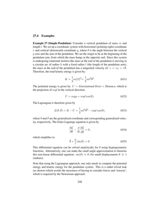
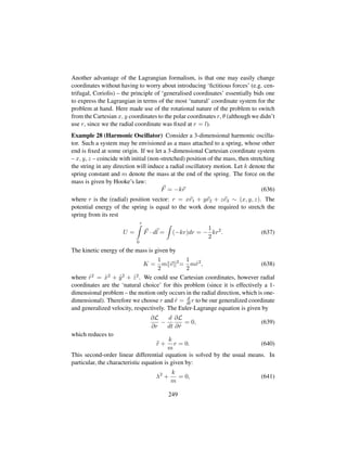
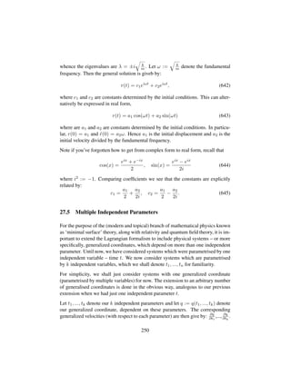
![Given some function L := L(q, ∂q
∂t1
, ..., ∂q
∂tk
; t1, ..., tk) explicitly dependent on the
generalized coordinate q, generalized velocities ∂q
∂ti
and implicitly dependent on the
independent parameters t1, ..., tk, we now wish to formulate a variational problem.
In particular, we consider the following action functional (a k-dimensional integral
performed over t1, ..., tk):
S[L] = Ldt1dt2...dtk (646)
and ask the question – which functions L make this action stationary? To solve the
variational problem, we proceed as before to vary the action by Taylor expansion
of L in all its variables. In order to do this, some new notation will be handy. Let vq
i
denote the i − th generalized velocity corresponding to the generalized coordinate
q – particular, we have: vq
1 := ∂q
∂t1
, ..., vq
k := ∂q
∂tk
. The variation of the Lagrangian
is then given using the same rules as the total differential:
δL =
∂L
∂q
δq +
∂L
∂vq
1
δvq
1 + ... +
∂L
∂vq
k
δvq
k. (647)
Therefore, the variation of the action is given by:
δS = δLdt1...dtk
= [
∂L
∂q
δq +
∂L
∂vq
1
δvq
1 + ... +
∂L
∂vq
k
δvq
k]dt1...dtk
= [
∂L
∂q
δq −
∂
∂t1
(
∂L
∂vq
1
)δq − ... −
∂
∂tk
(
∂L
∂vq
k
)δq]dt1...dtk
= [
∂L
∂q
−
∂
∂t1
(
∂L
∂vq
1
) − ... −
∂
∂tk
(
∂L
∂vq
k
)]δqdt1...dtk. (648)
where we have used integration by parts (or Stoke’s Theorem) for multiple vari-
ables, to swap the derivatives ∂
∂ti
from the velocity variations δ ∂q
∂ti
to the corre-
sponding coefficients ∂q
∂ti
– which introduces the minus signs. Therefore, we have
the functional derivative of the action with respect to the generalized coordinate,
given by:
δS
δq
=
∂L
∂q
−
∂
∂t1
(
∂L
∂vq
1
) − ... −
∂
∂tk
(
∂L
∂vq
k
). (649)
The principal of stationary action tells us that nature classically selects this func-
tional derivative to be zero, which gives us the Euler-Lagrange equations for a sys-
tem with one generalized coordinate q, parametrised by k independent variables
t1, ..., tk:
0 =
δS
δq
|Nature=
∂L
∂q
−
∂
∂t1
(
∂L
∂vq
1
) − ... −
∂
∂tk
(
∂L
∂vq
k
). (650)
251](https://image.slidesharecdn.com/1f3b3f2a-4e32-4167-891e-7d7de5f1c671-150709175058-lva1-app6892/85/SGC-2014-Mathematical-Sciences-Tutorials-251-320.jpg)
![27.6 More Examples
We can use variational calculus to derive the (rather famous) minimal surface equa-
tion. In particular, we consider the following example.
Example 29 (Minimal Surface Equation) We consider all two-dimensional sur-
faces parametrised by two independent variables, z := z(x, y), then ask the ques-
tion – which surface of this general form has the minimal surface area? To answer
this question, we can use the Euler-Lagrange equation (650) derived earlier. Say
that the surface z := z(x, y) parametrised by the two independent variables t1 = x
and t2 = y, has a domain D. Then (recall) its surface area is given by the double-
integral:
A =
d
1 + (
∂z
∂x
)2 + (
∂z
∂y
)2dxdy. (651)
We can view this as a variational problem by observing that: z is generalised co-
ordinate parametrised by two independent variables x and y. The correspond-
ing generalised velocities are given by (various notations) vz
1 = zx := ∂z
∂x and
vz
2 = zy := ∂z
∂y – we shall stick with the latter notation. Now, the total surface
area A can be viewed as an action functional: A = A[L], whilst our integrand
(infinitesimal / area differential) can be viewed as the corresponding Lagrangian:
L(z, zx, zy) =
˜
1 + (∂z
∂x )2 + (∂z
∂y )2 =
˜
1 + z2
x + z2
y.
Since we seek to minimize A, we need to first find surfaces (parametric functions)
z(x, y) which make the functional A stationary. We then need to check that these
stationary ‘points’ (functions) correspond to minima, rather than inflection points
or maxima. The first task can be achieved by solving the Euler-Lagrange equations
(650), which take the form:
∂L
∂z
−
d
dx
∂L
∂zx
−
d
dy
L
∂zy
=0 =⇒
0 +
d
dx
zx
˜
1 + z2
x + z2
y
+
d
dy
zy
˜
1 + z2
x + z2
y
=0 . (652)
Although the last equation, known as the ‘minimal surface equation’, was derived
by Lagrange in 1762, non-trivial (non-planar) solutions were not found till 1776
by the French Mathematical Engineer, Jean Meusnier. In particular, the planar
solution is given by:
Z(x, y) = Ax + By + C (653)
where A, B, C are constants. Here Zx = ∂Z
∂x = A, Zy = ∂Z
∂y = B and L =
?
1 + A2 + B2 e.t.c.
252](https://image.slidesharecdn.com/1f3b3f2a-4e32-4167-891e-7d7de5f1c671-150709175058-lva1-app6892/85/SGC-2014-Mathematical-Sciences-Tutorials-252-320.jpg)