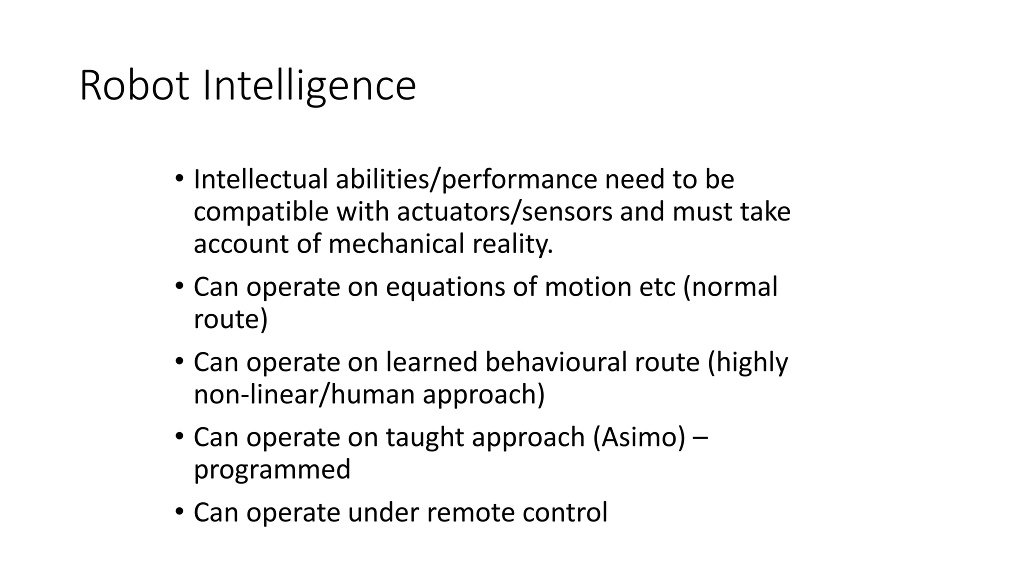
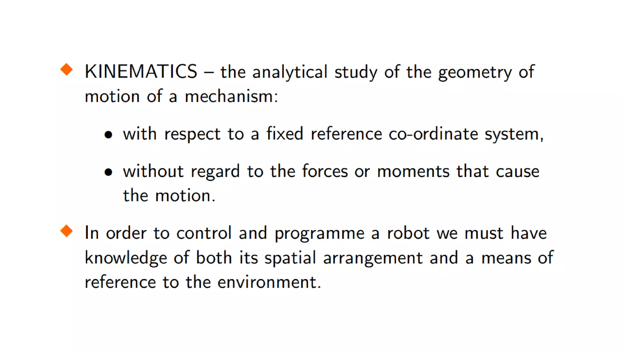
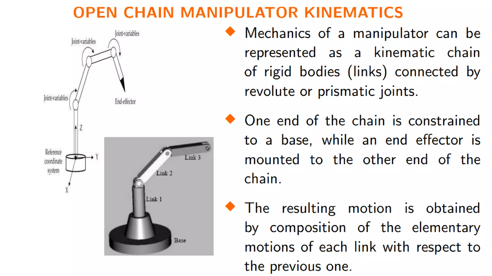
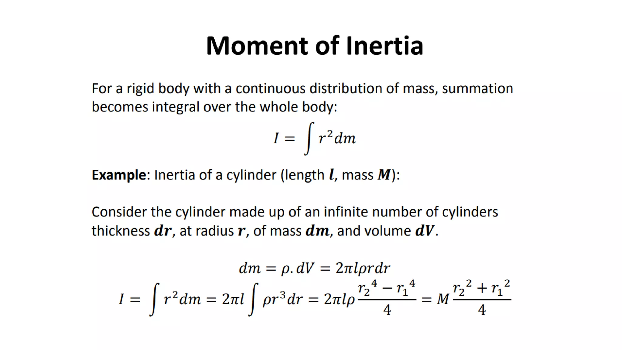
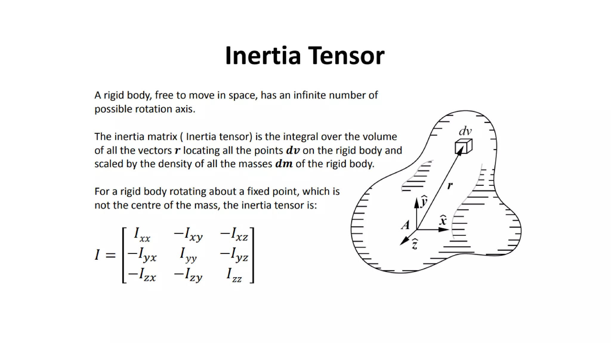
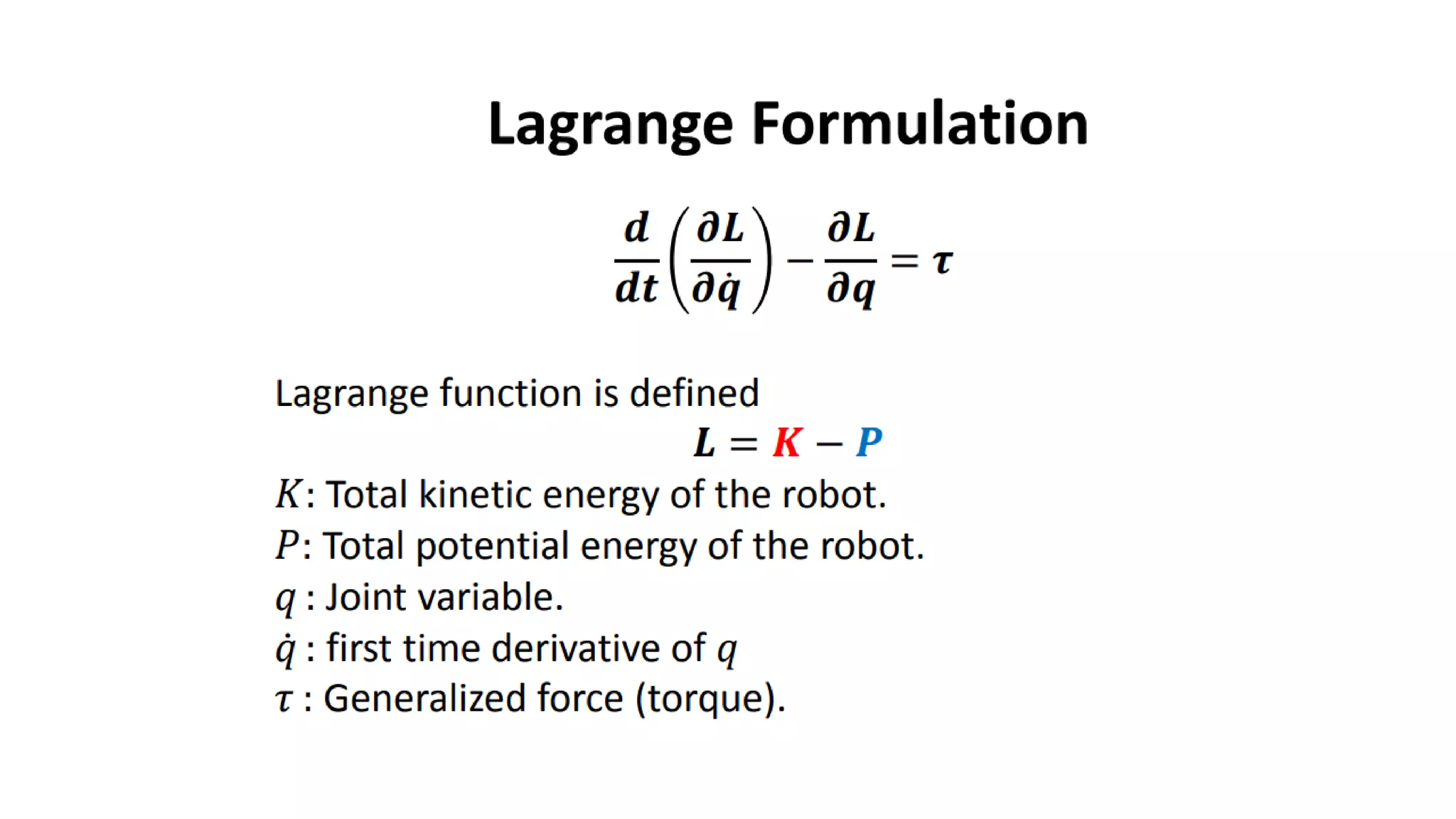
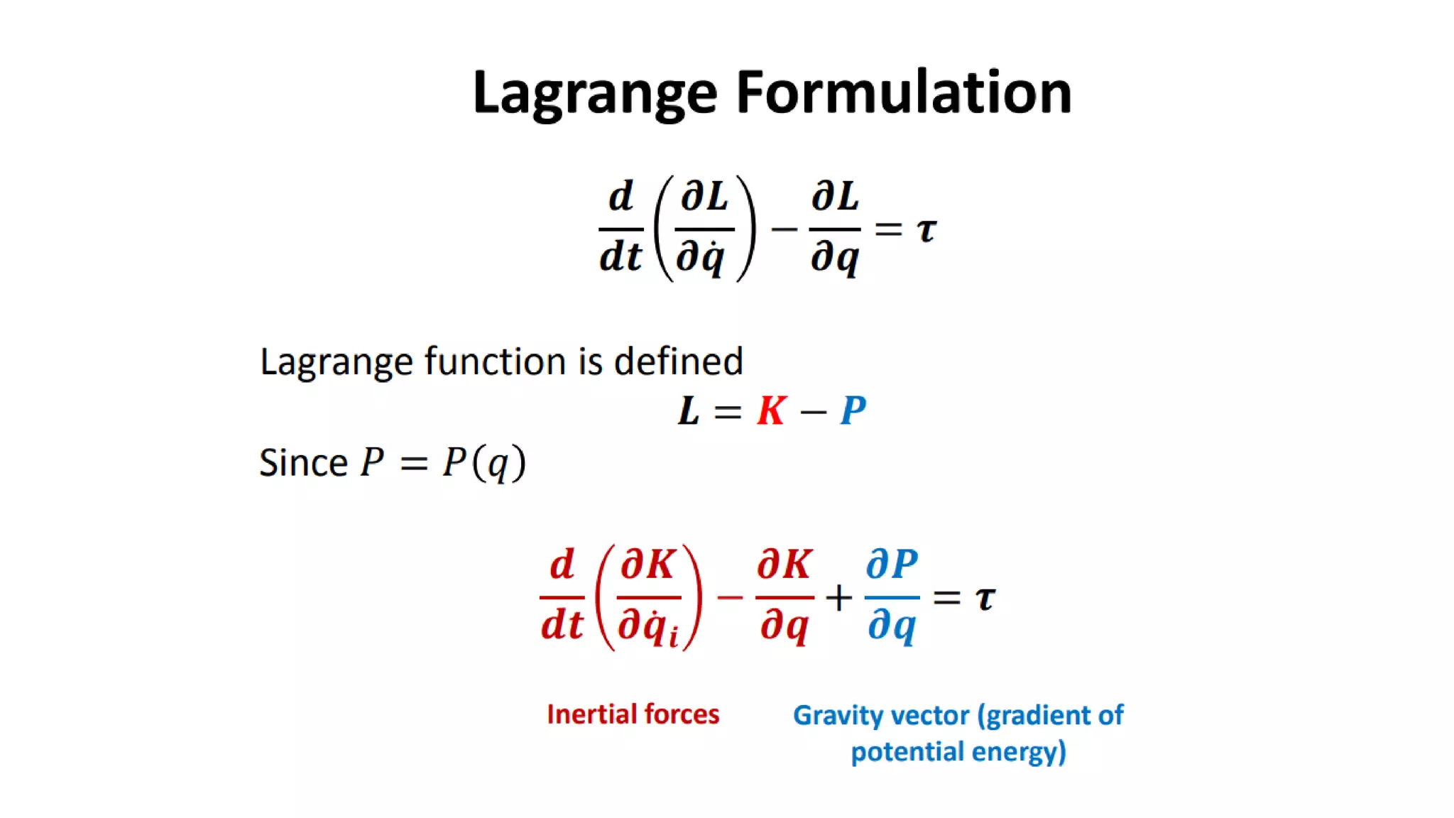
This document discusses robot kinematics and provides definitions and explanations of key terms:
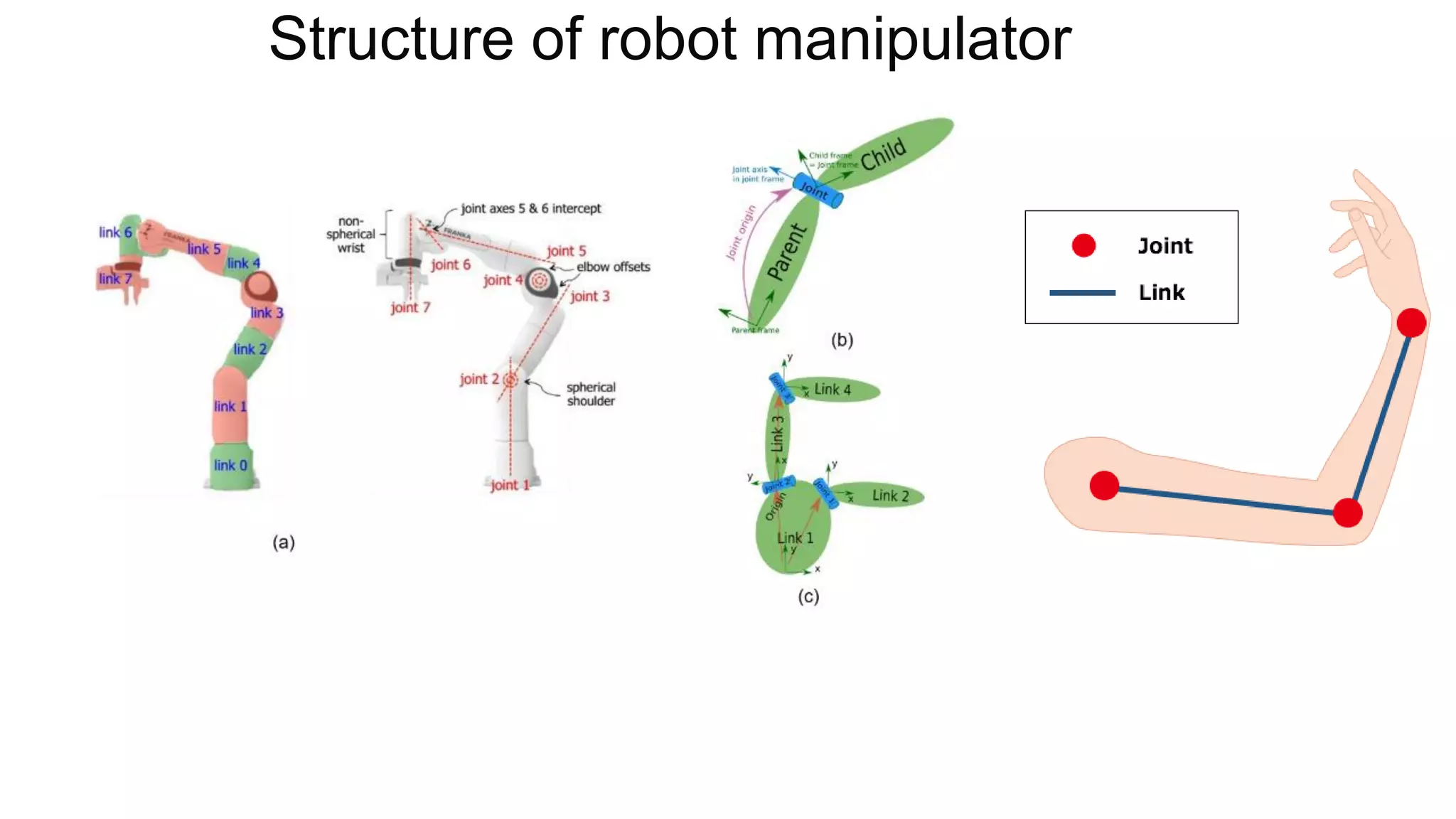
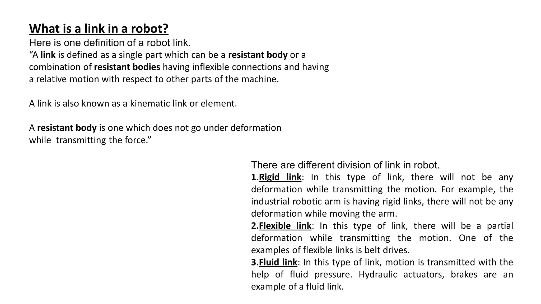
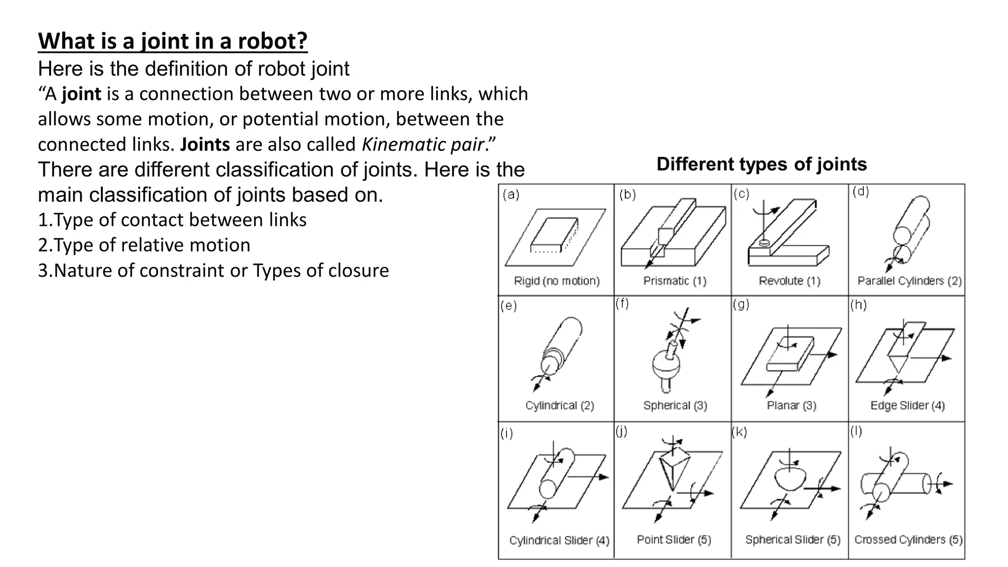
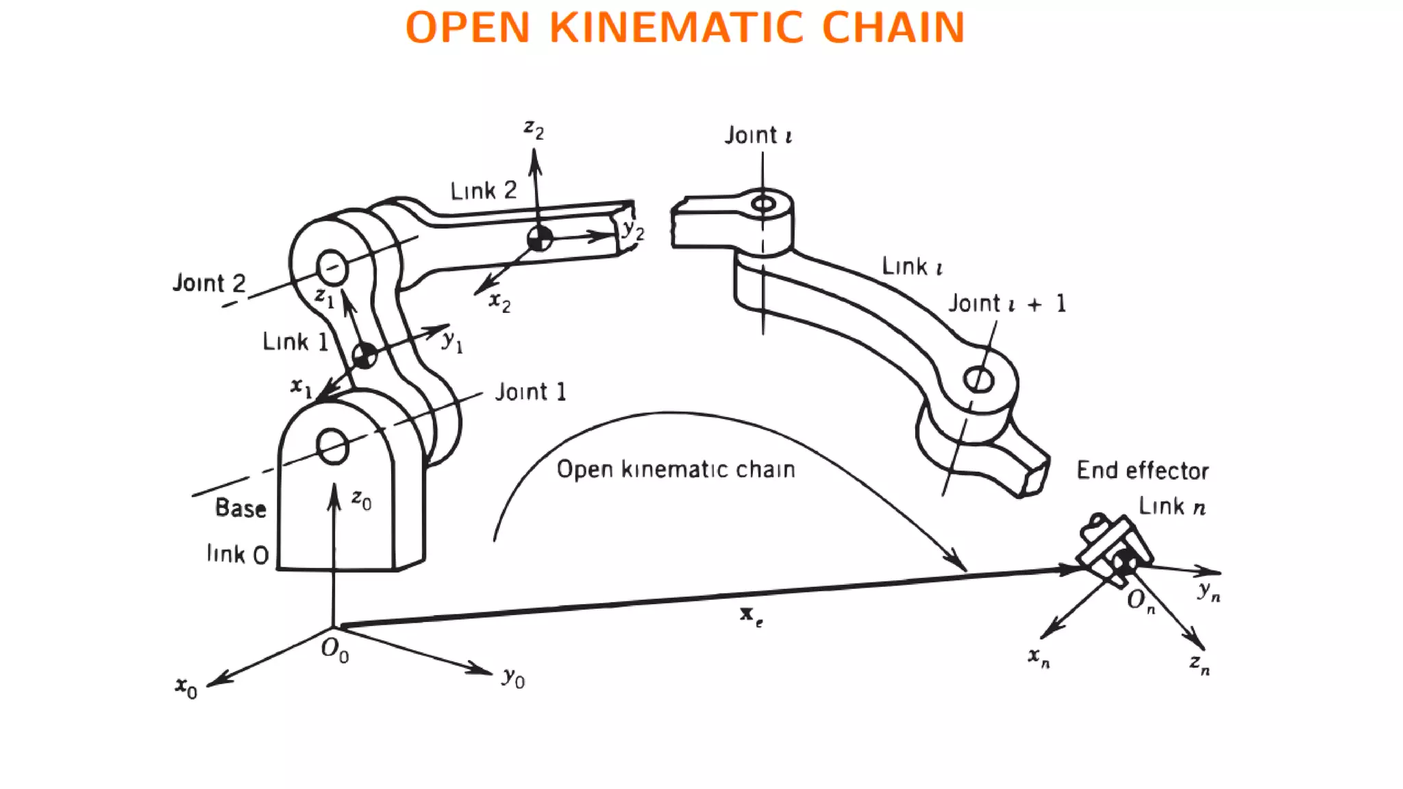
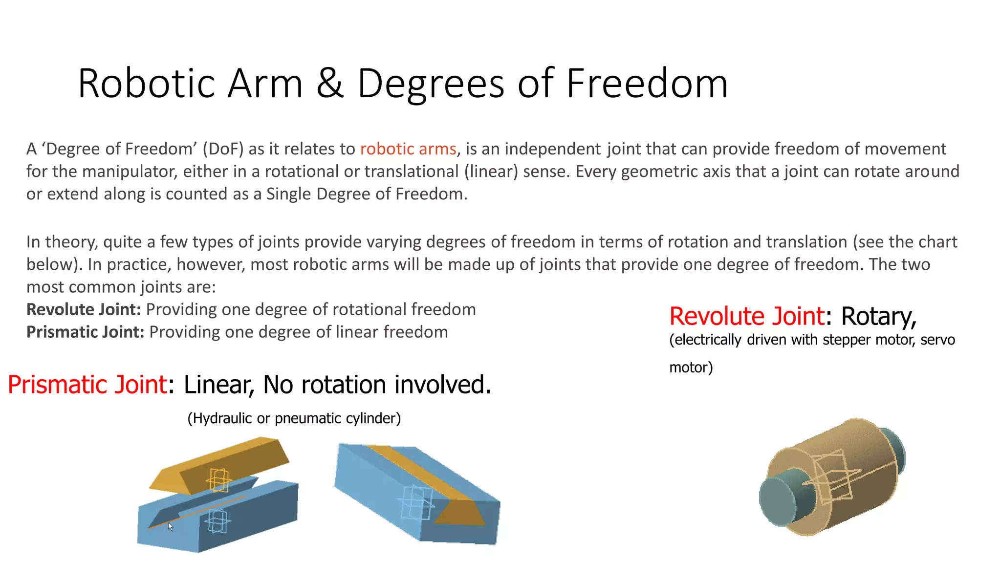
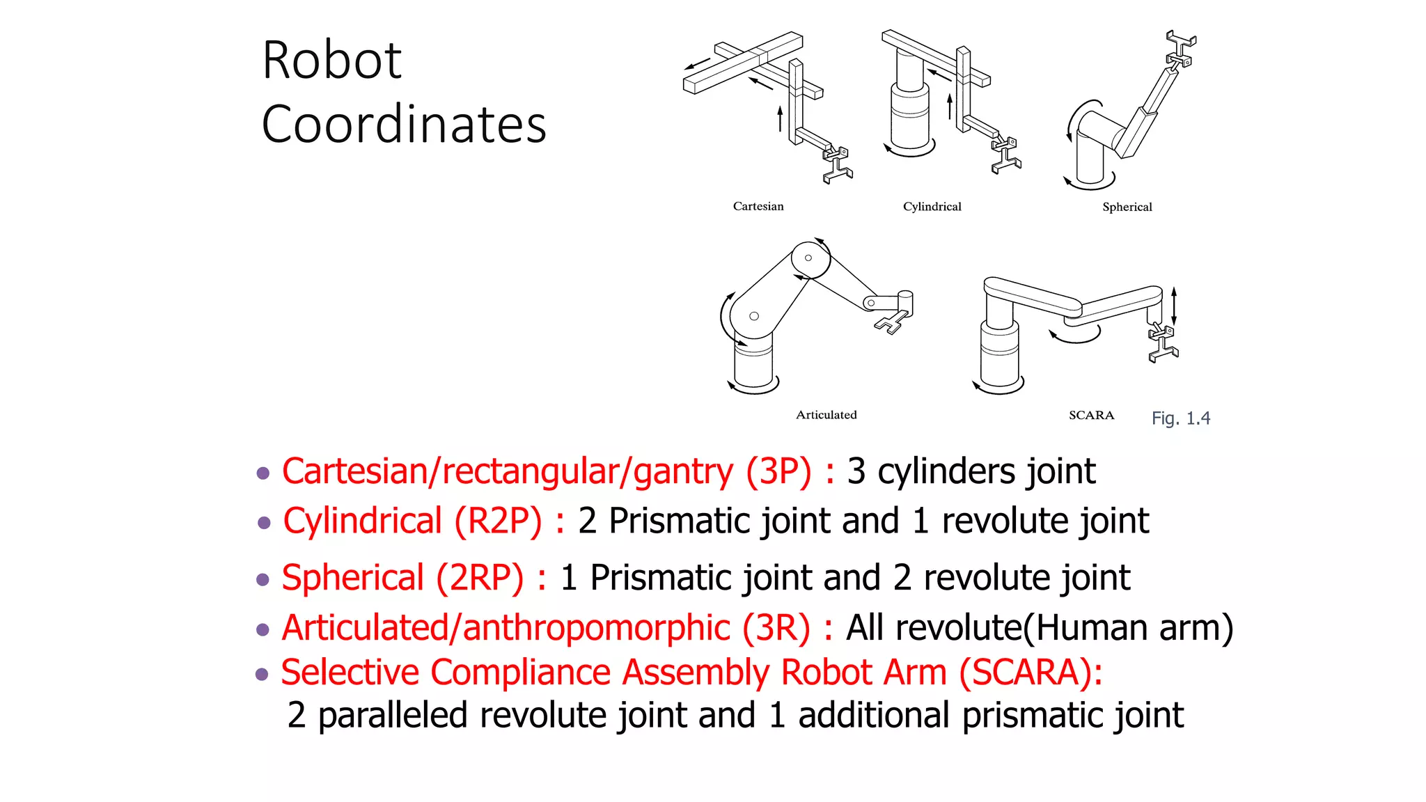
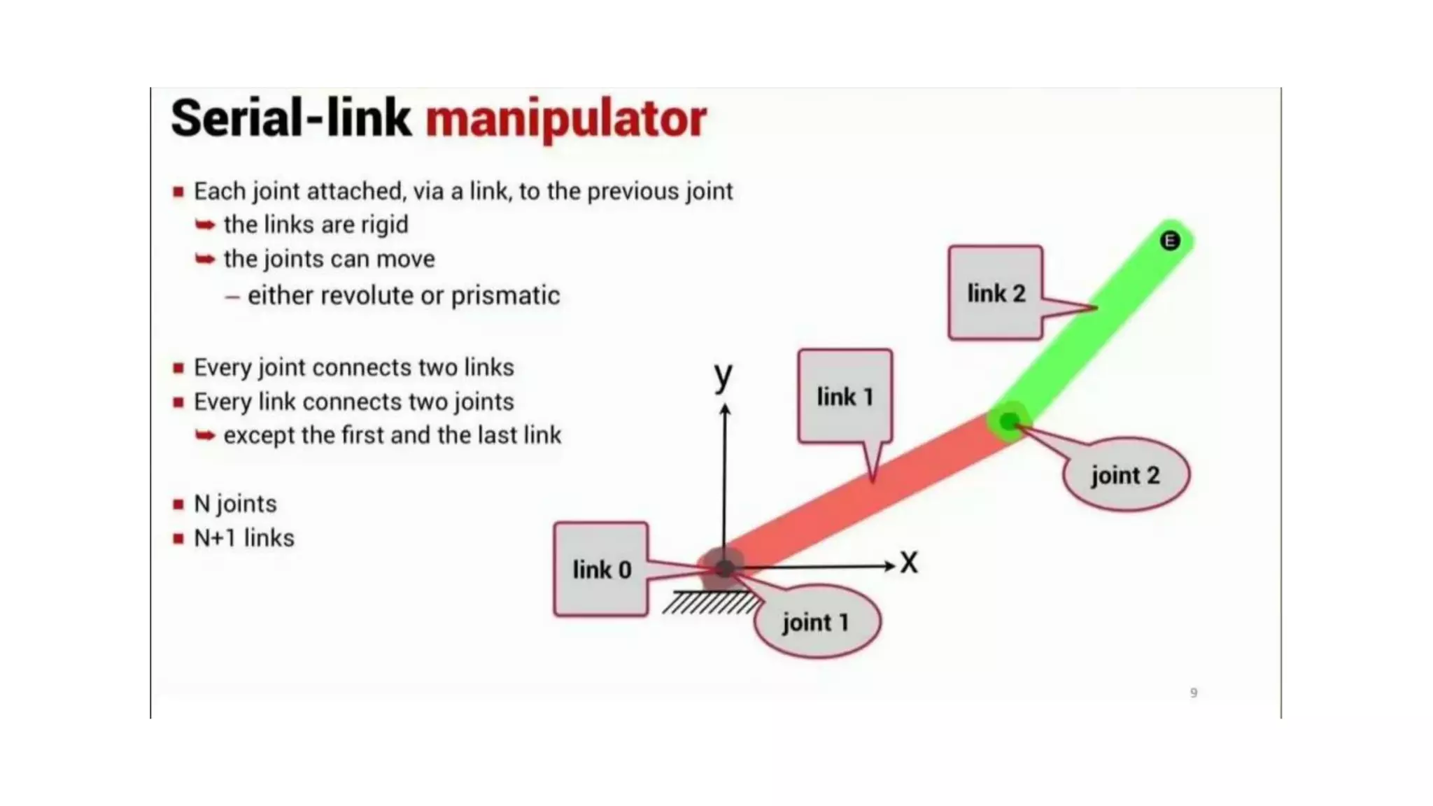
- A link is a rigid part of a robot that connects joints. Joints allow motion between connected links.
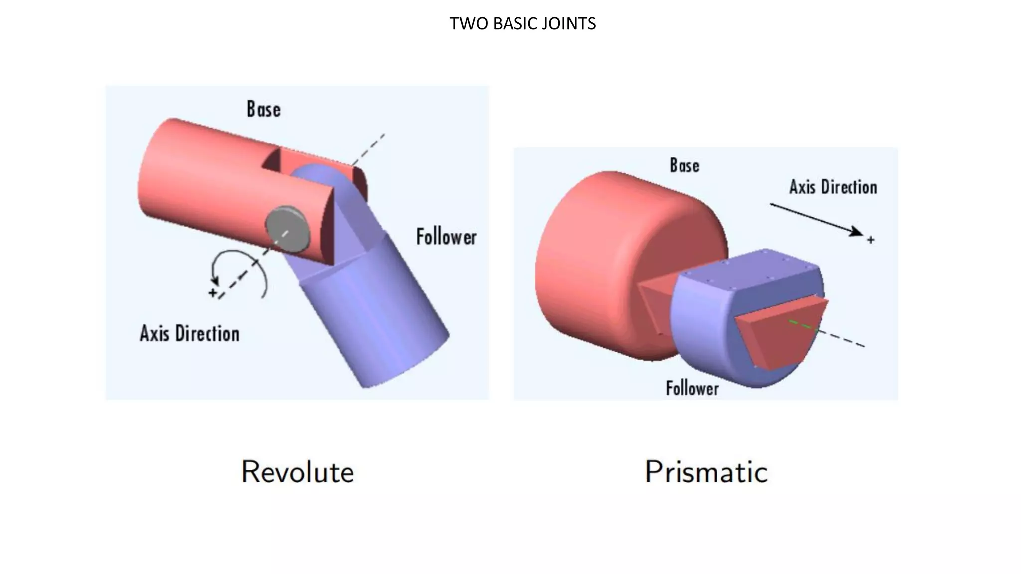
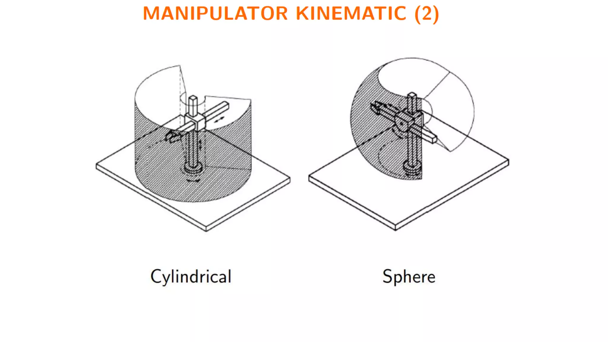
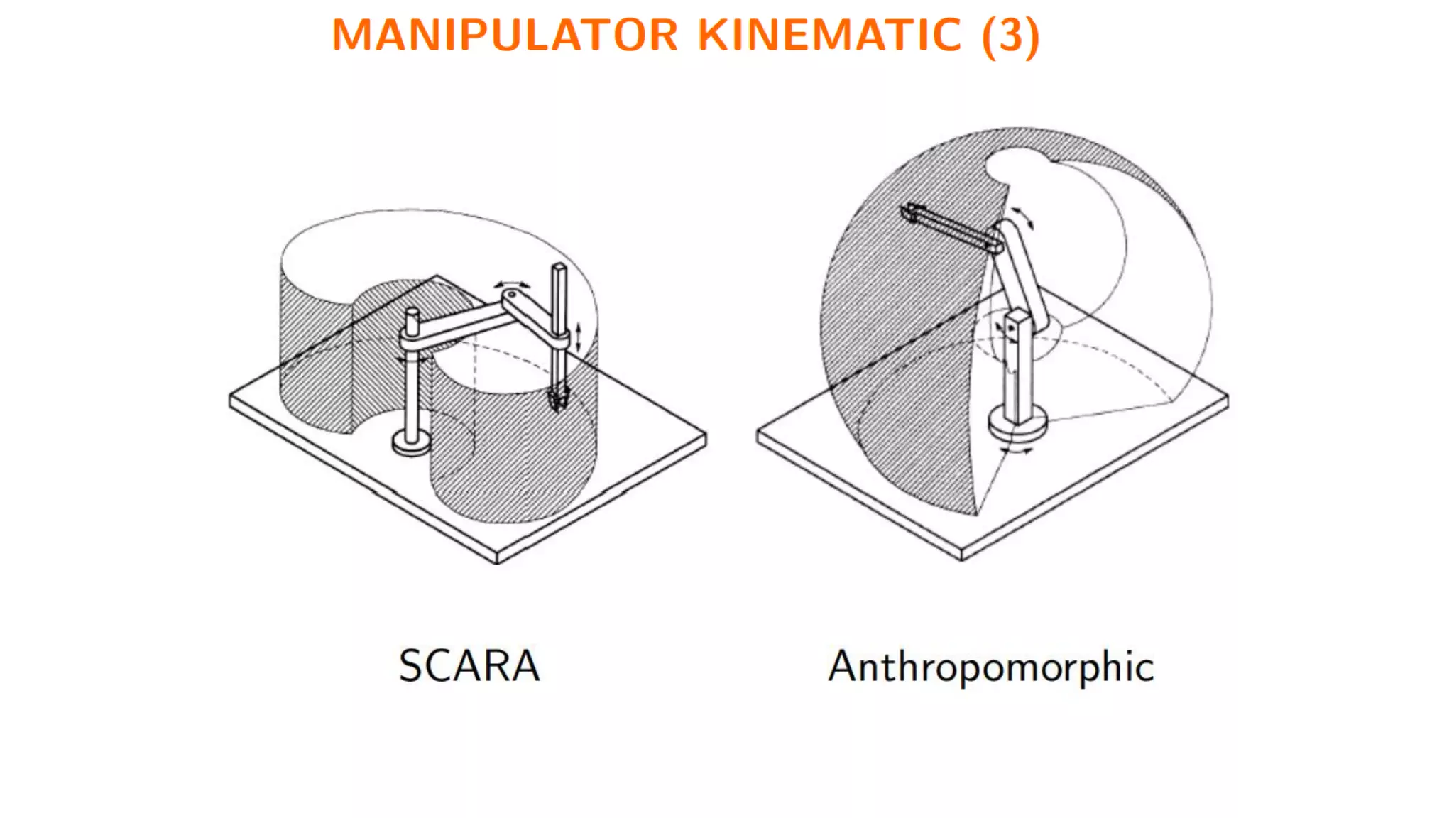
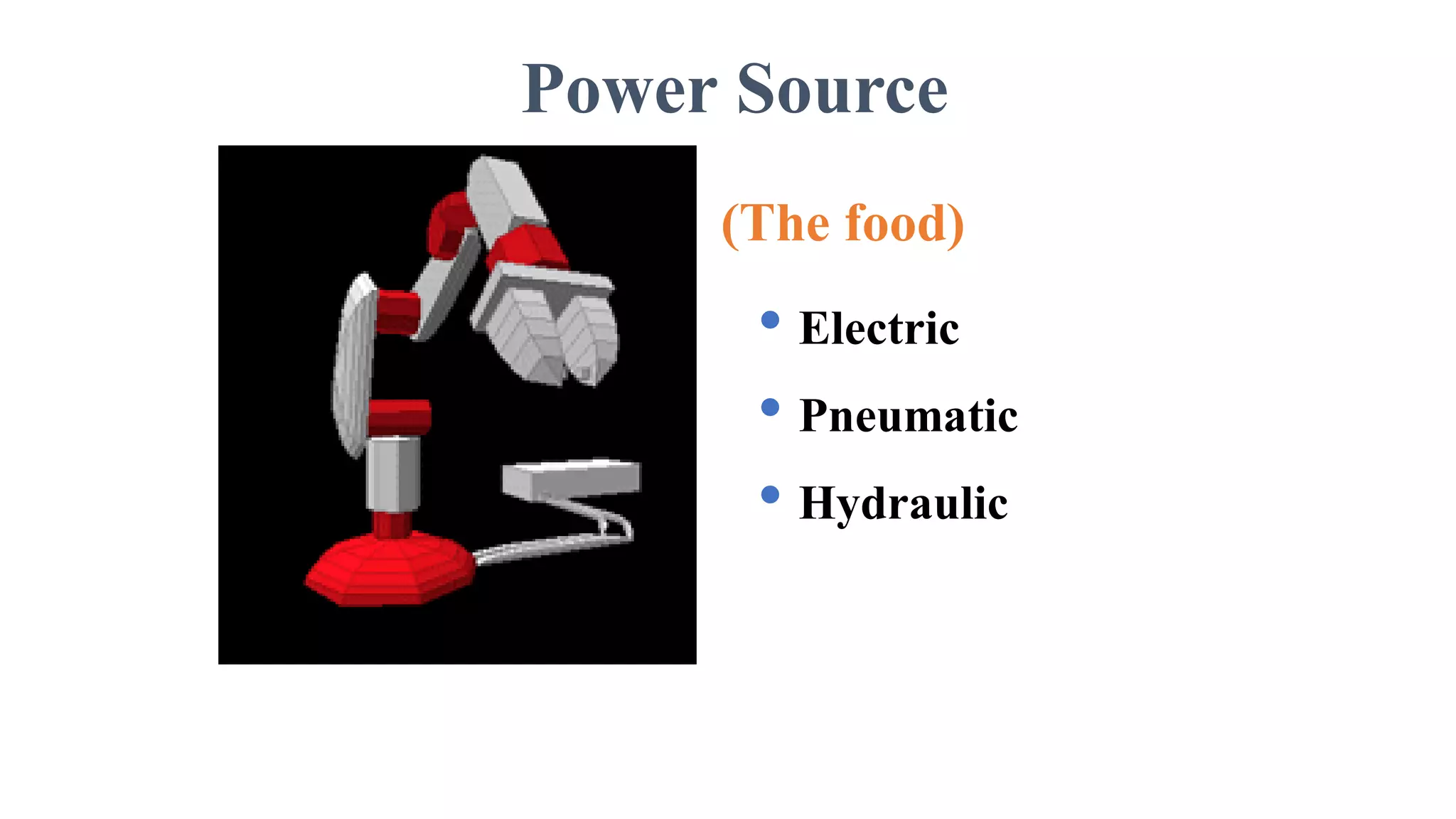
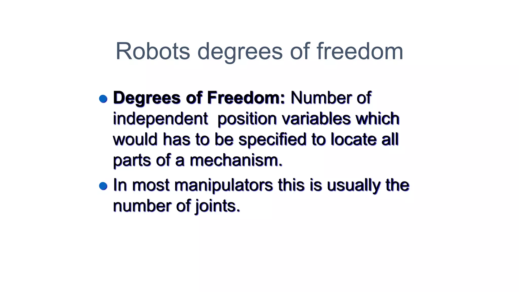
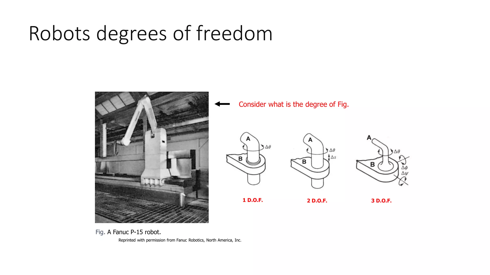
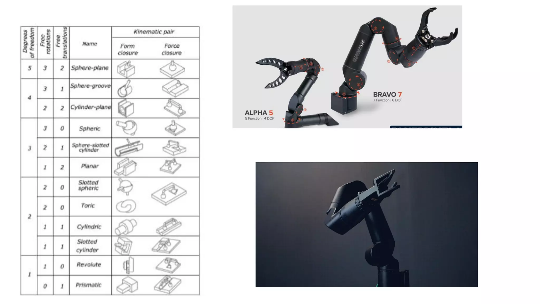
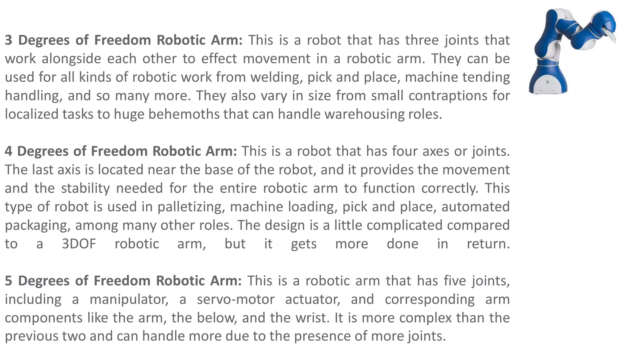
- There are different types of joints (revolute, prismatic, etc.) and each provides a degree of freedom (DOF) of motion.
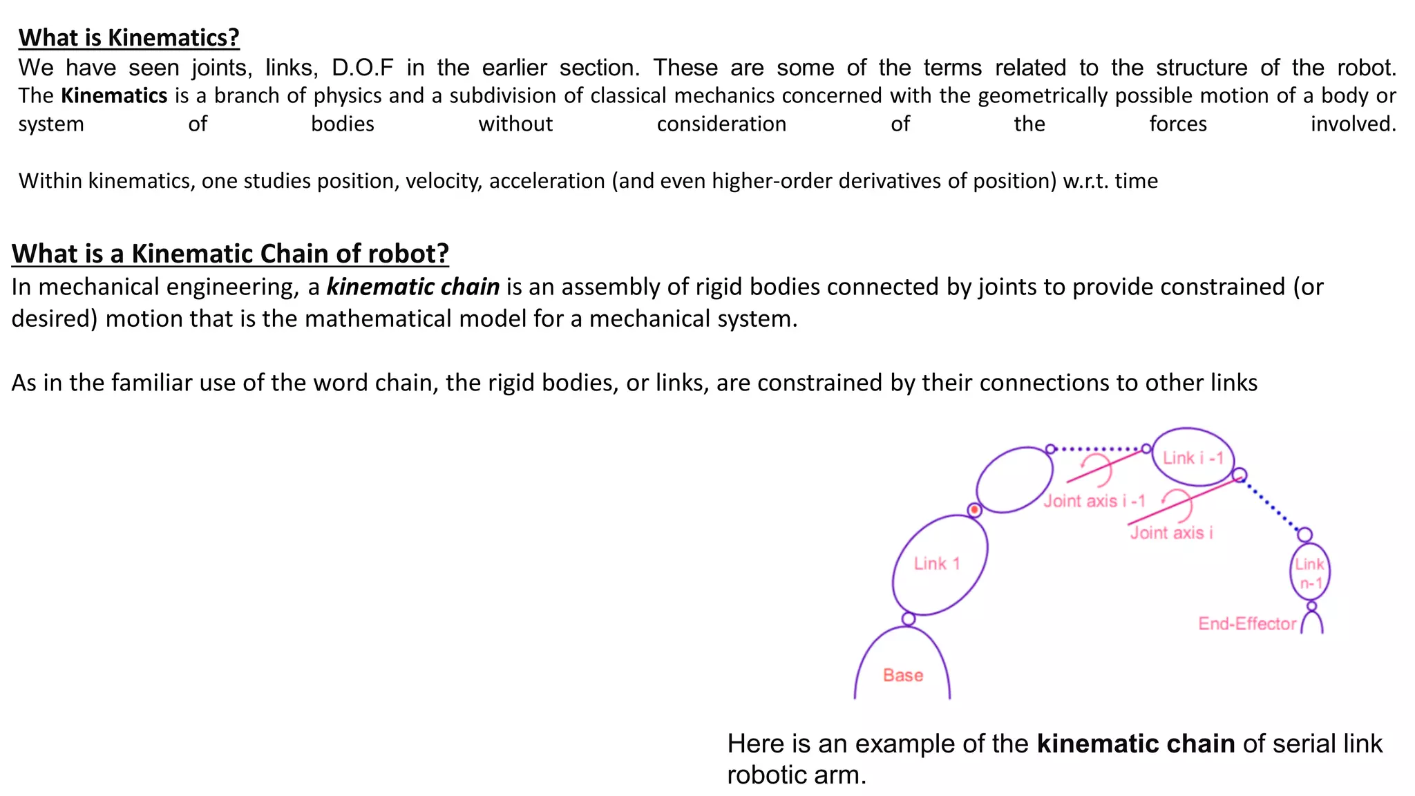
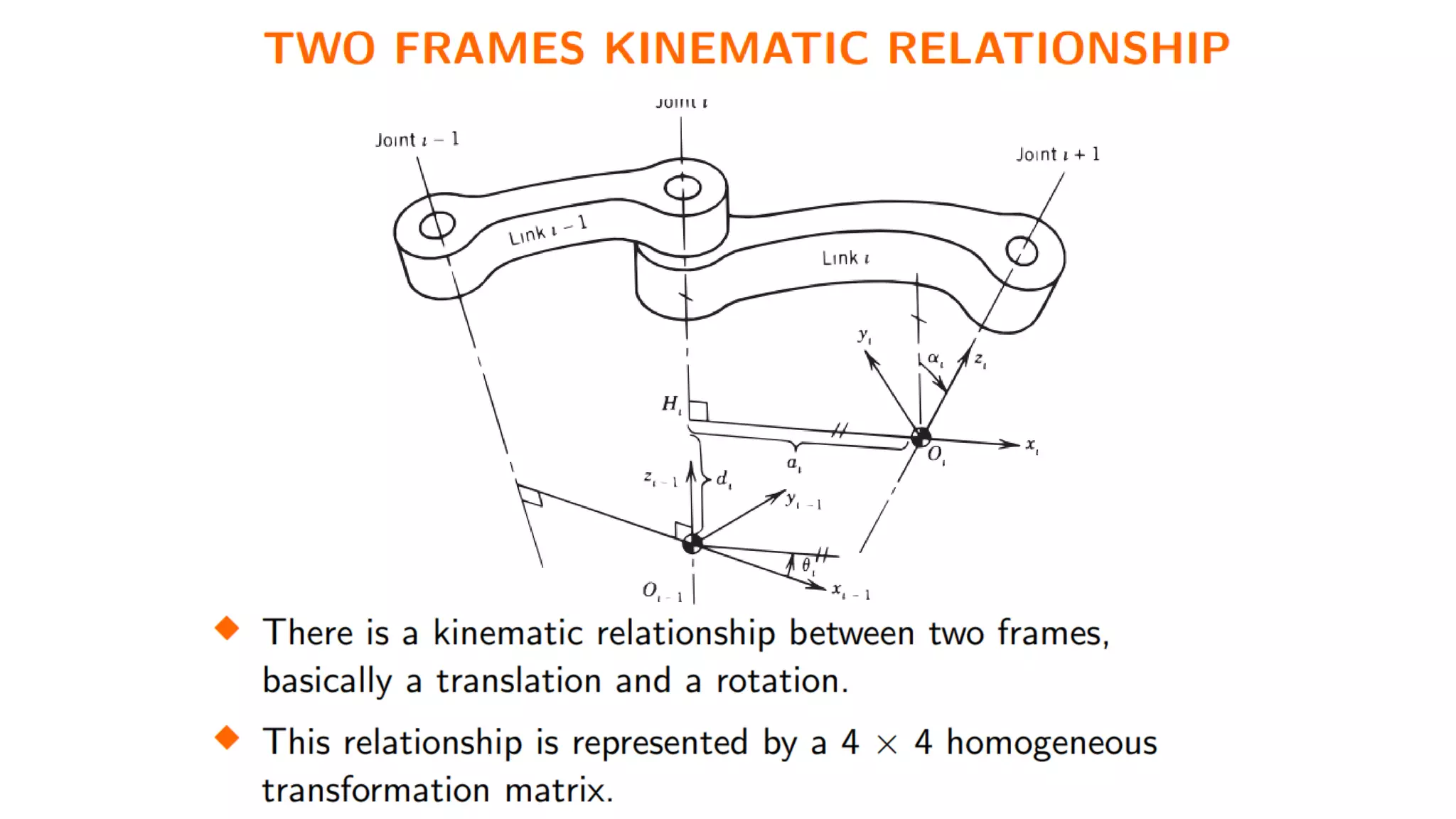
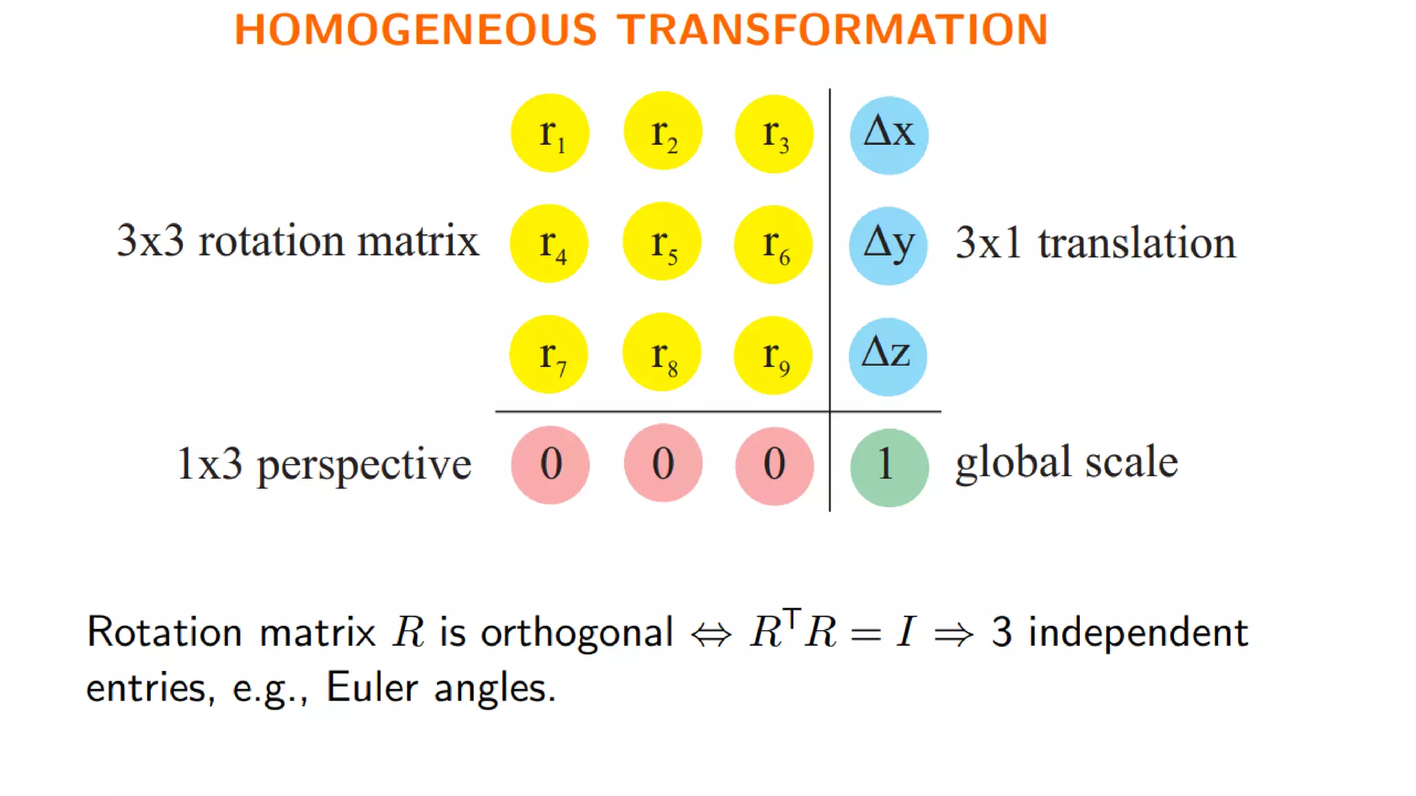
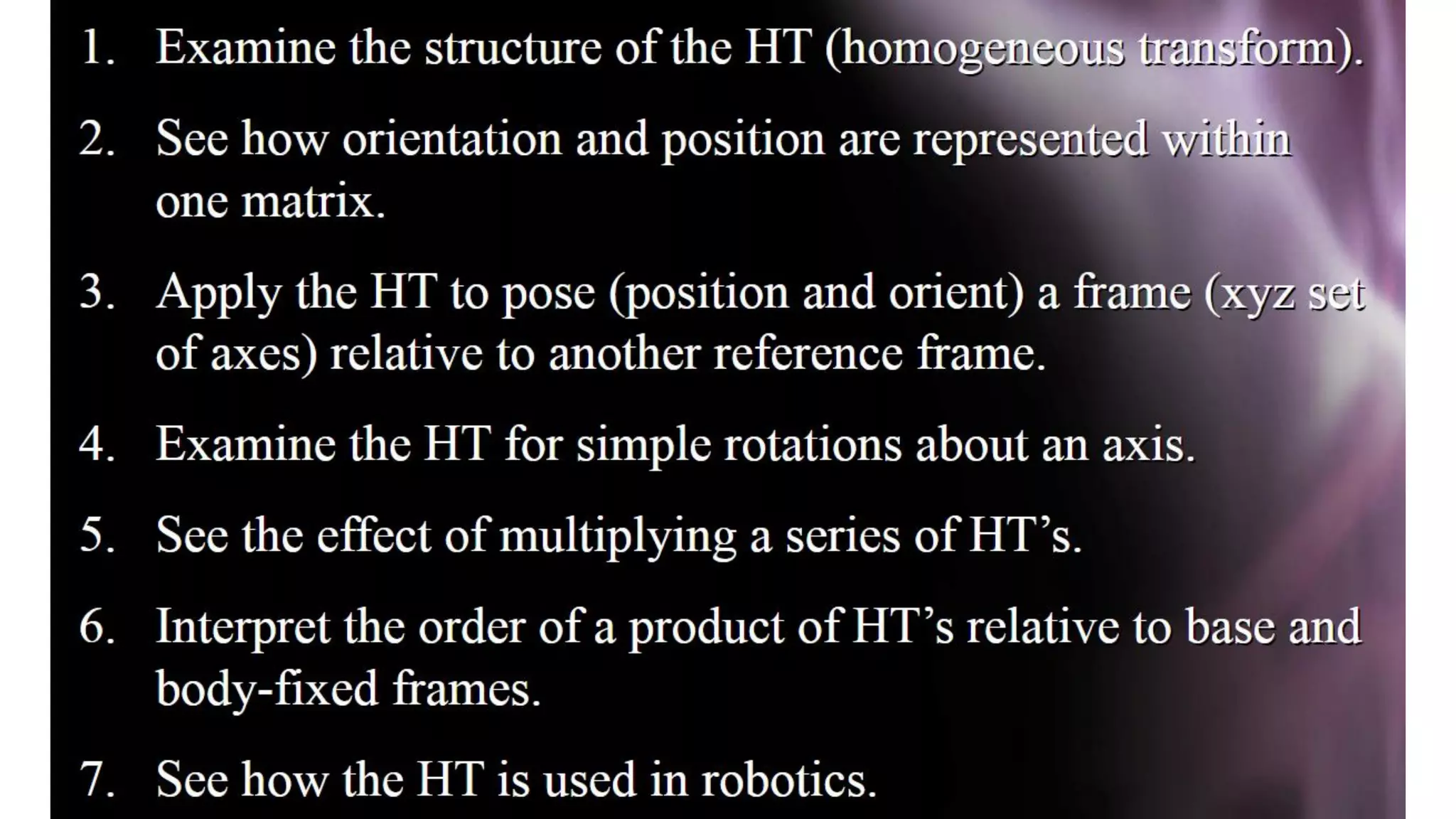
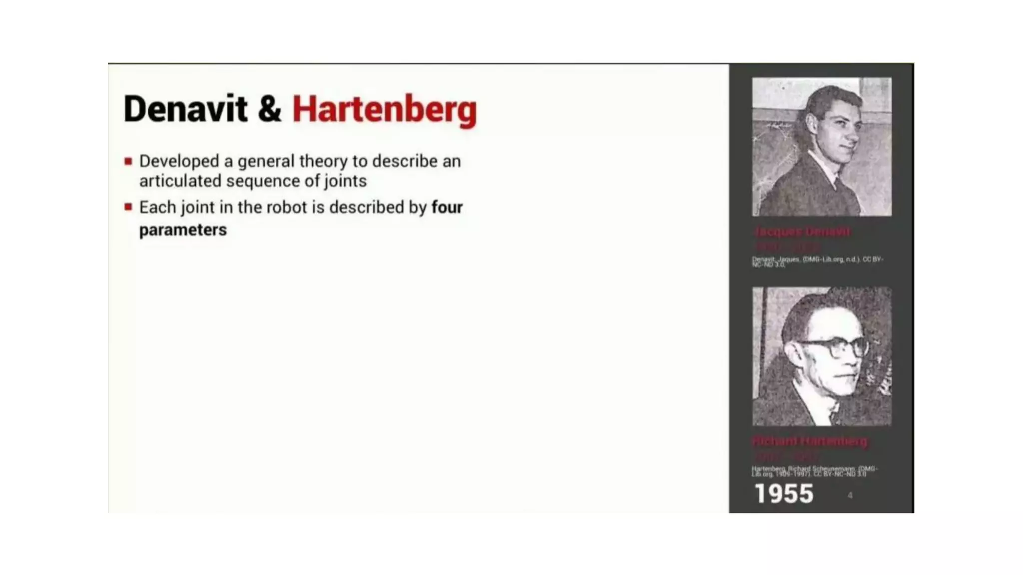
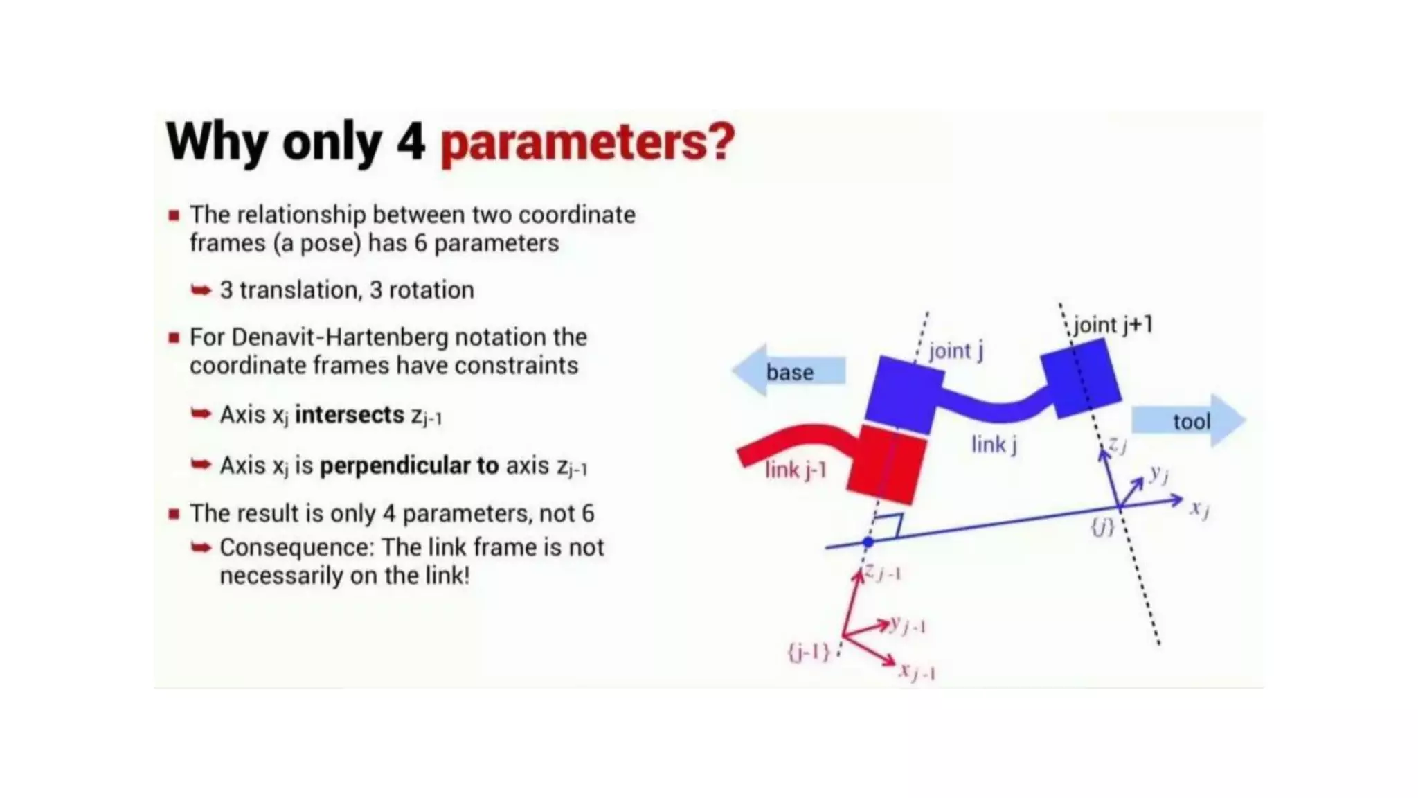
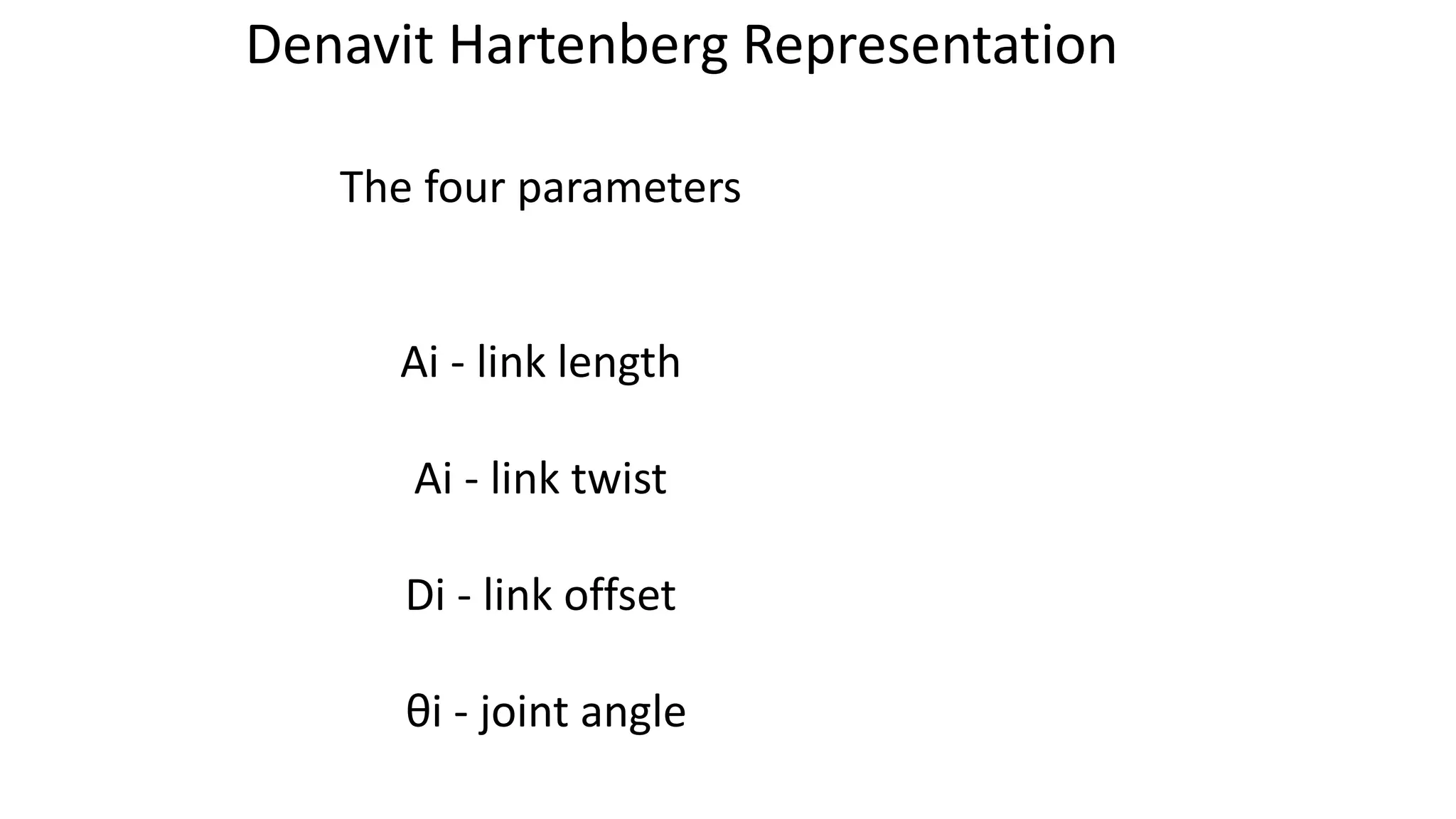
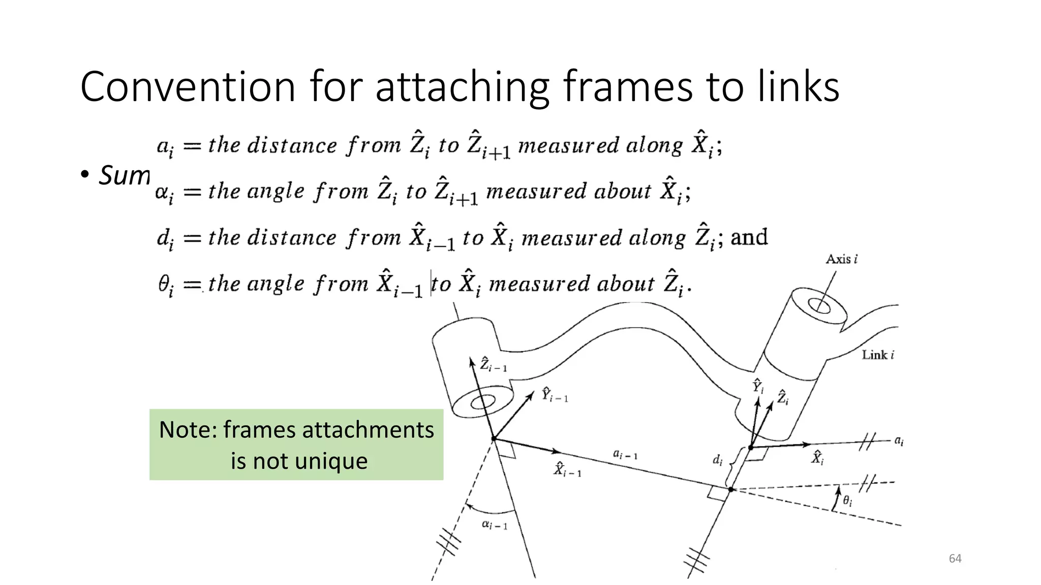
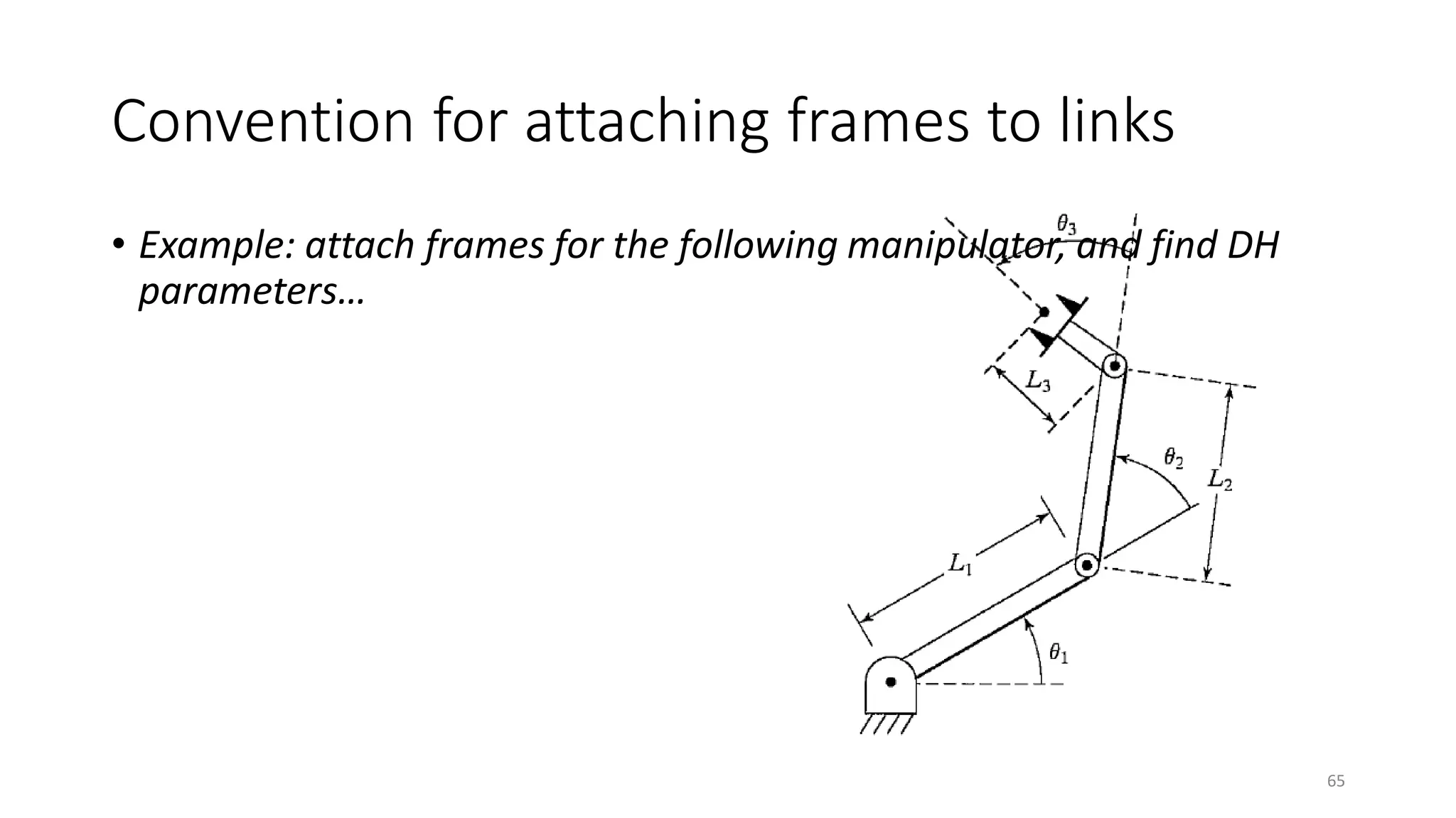
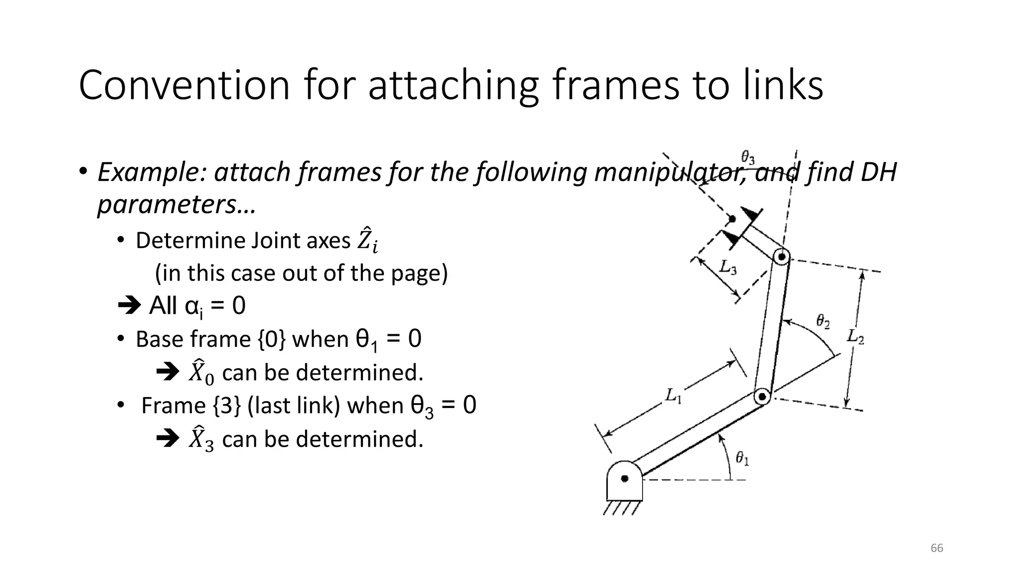
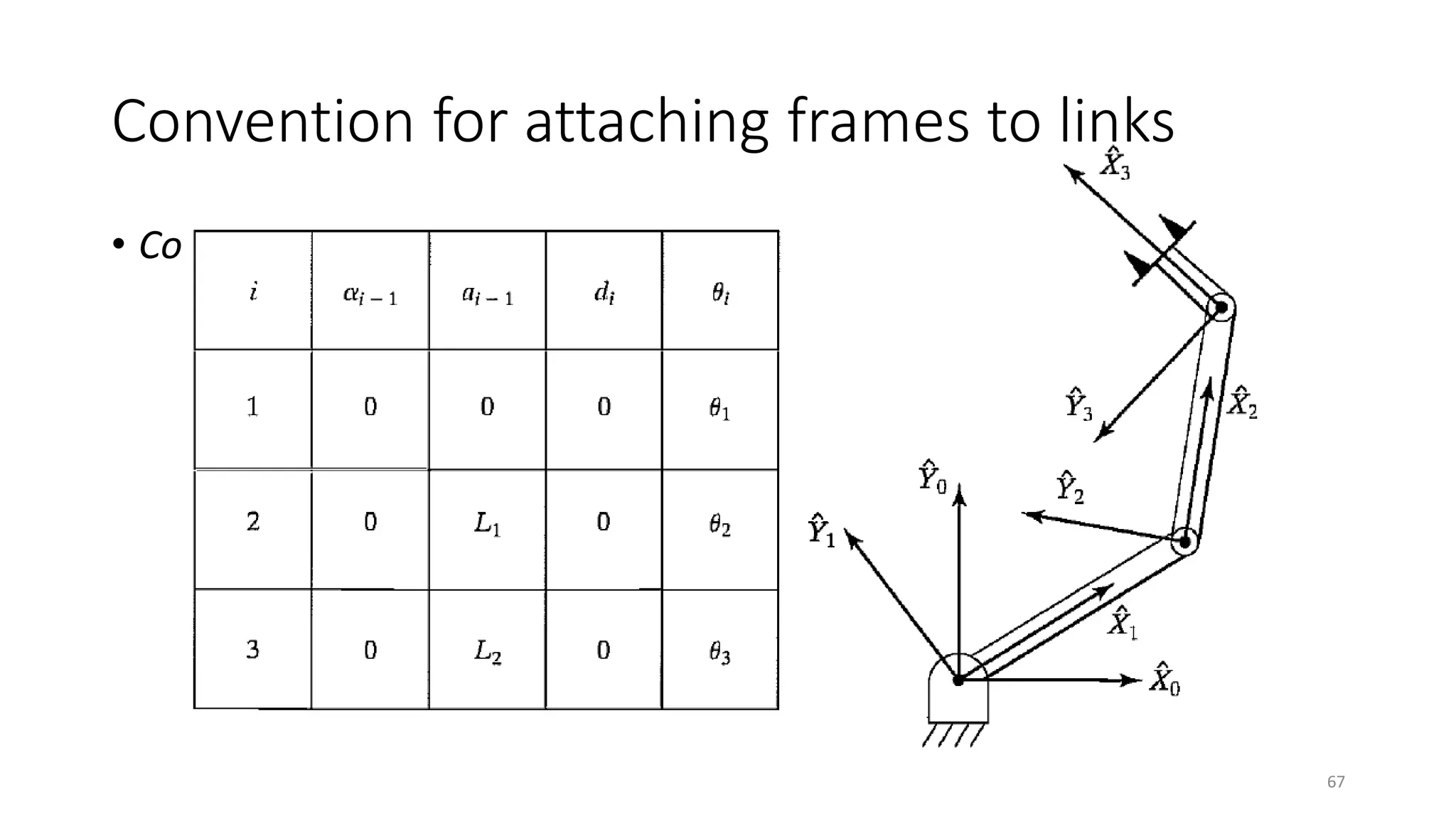
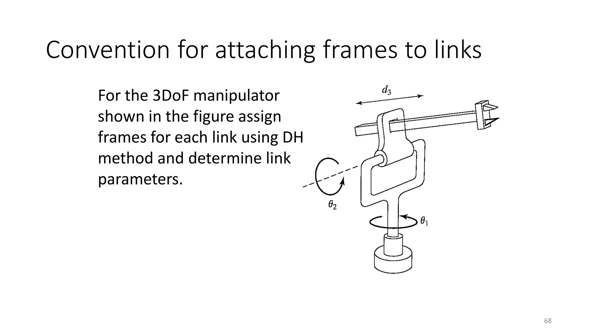
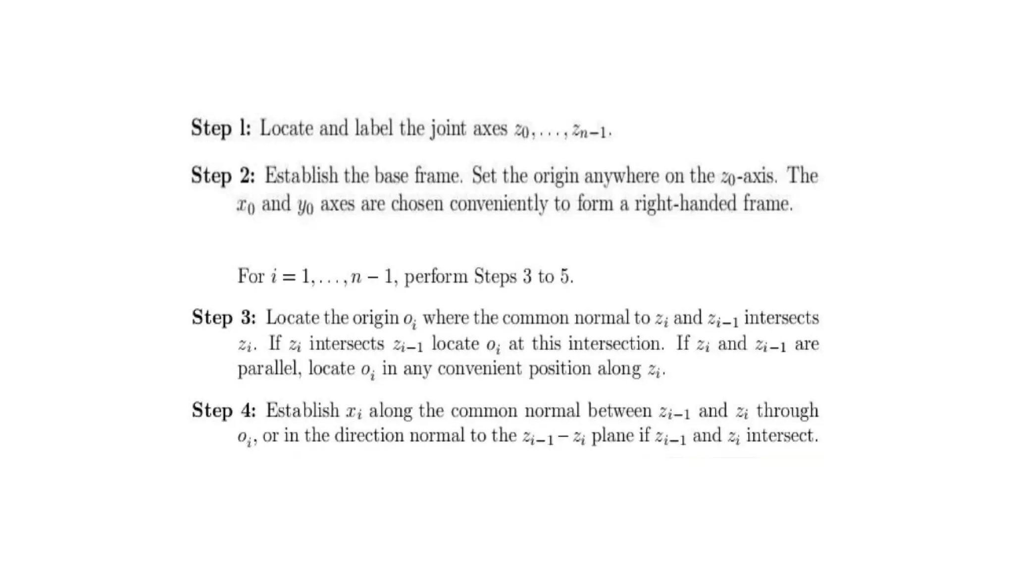
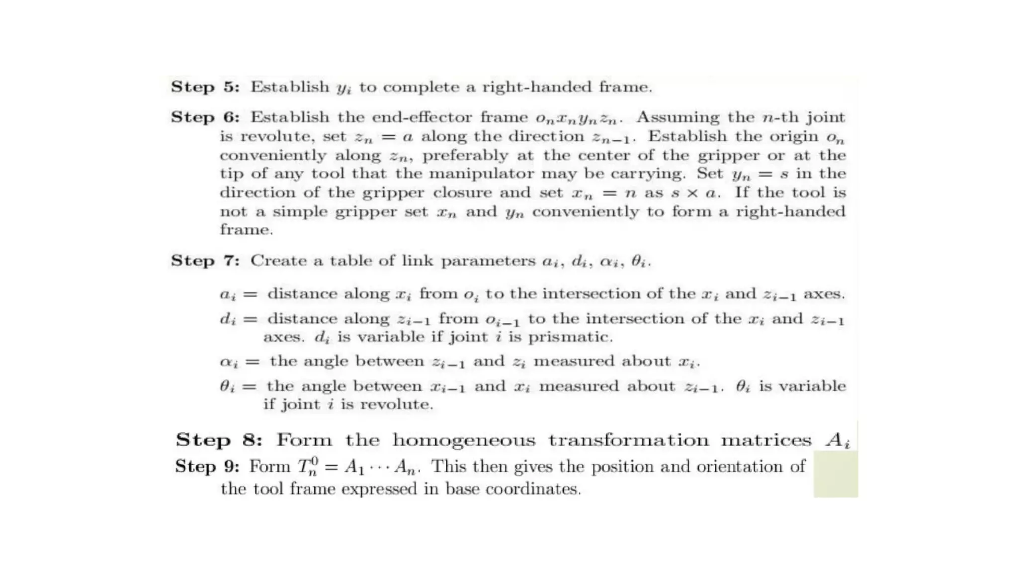
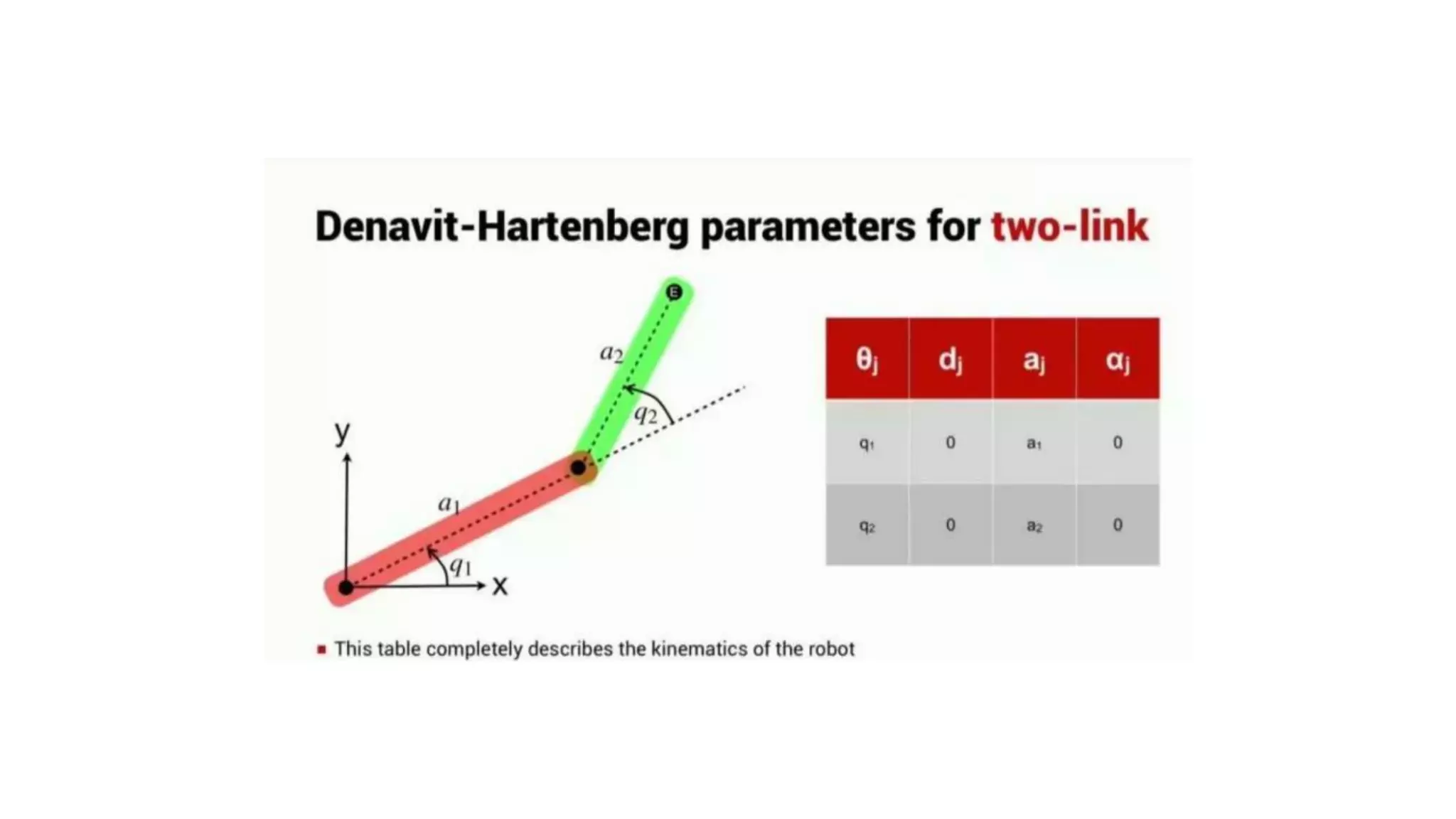
- The Denavit-Hartenberg (DH) convention defines a mathematical representation of a robot's kinematic structure using link parameters like link length, twist, offset and joint angle.
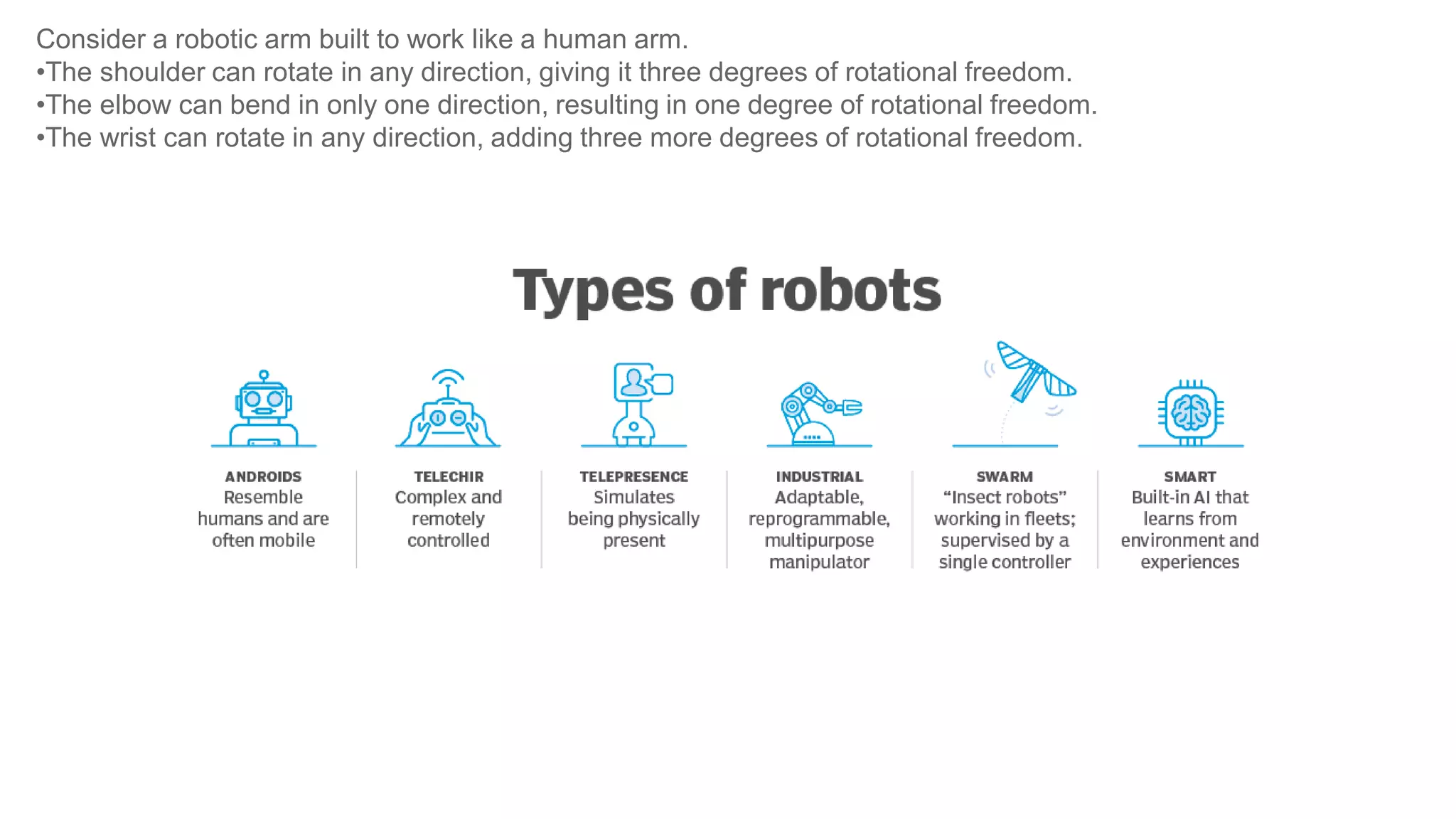
- A robot's degrees of freedom depend on the number and type of joints. Common robotic arm designs have between 3-7 DOF.


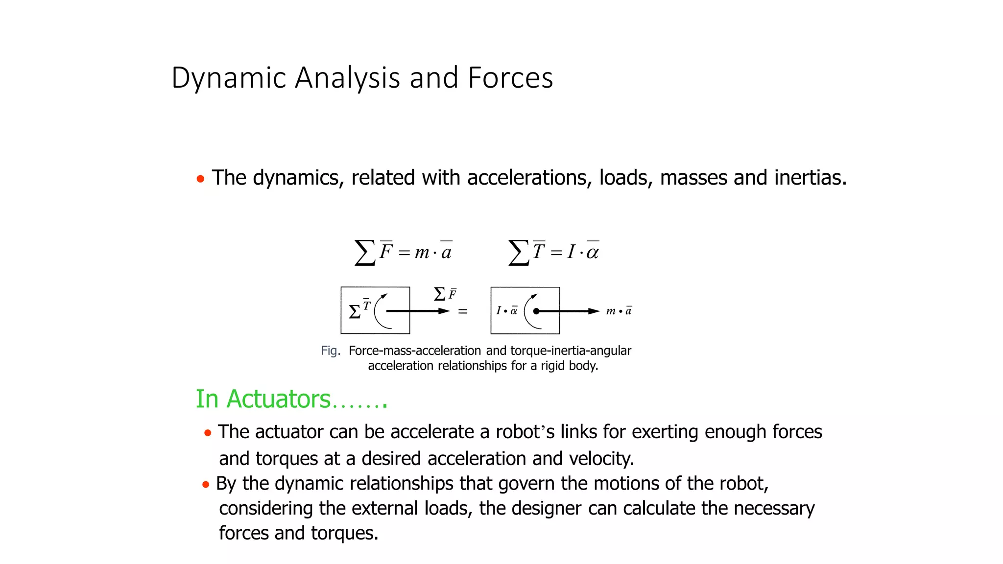


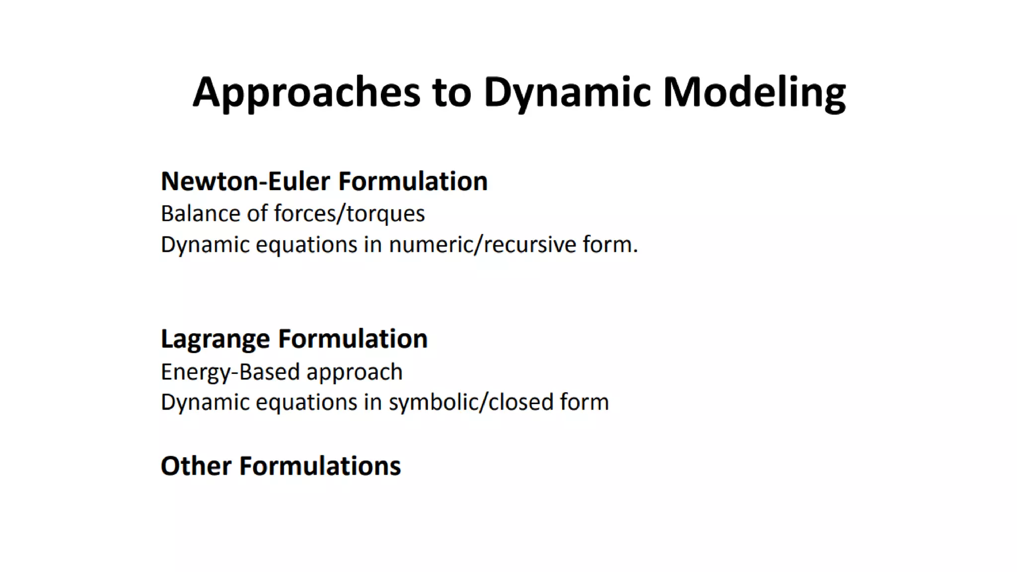
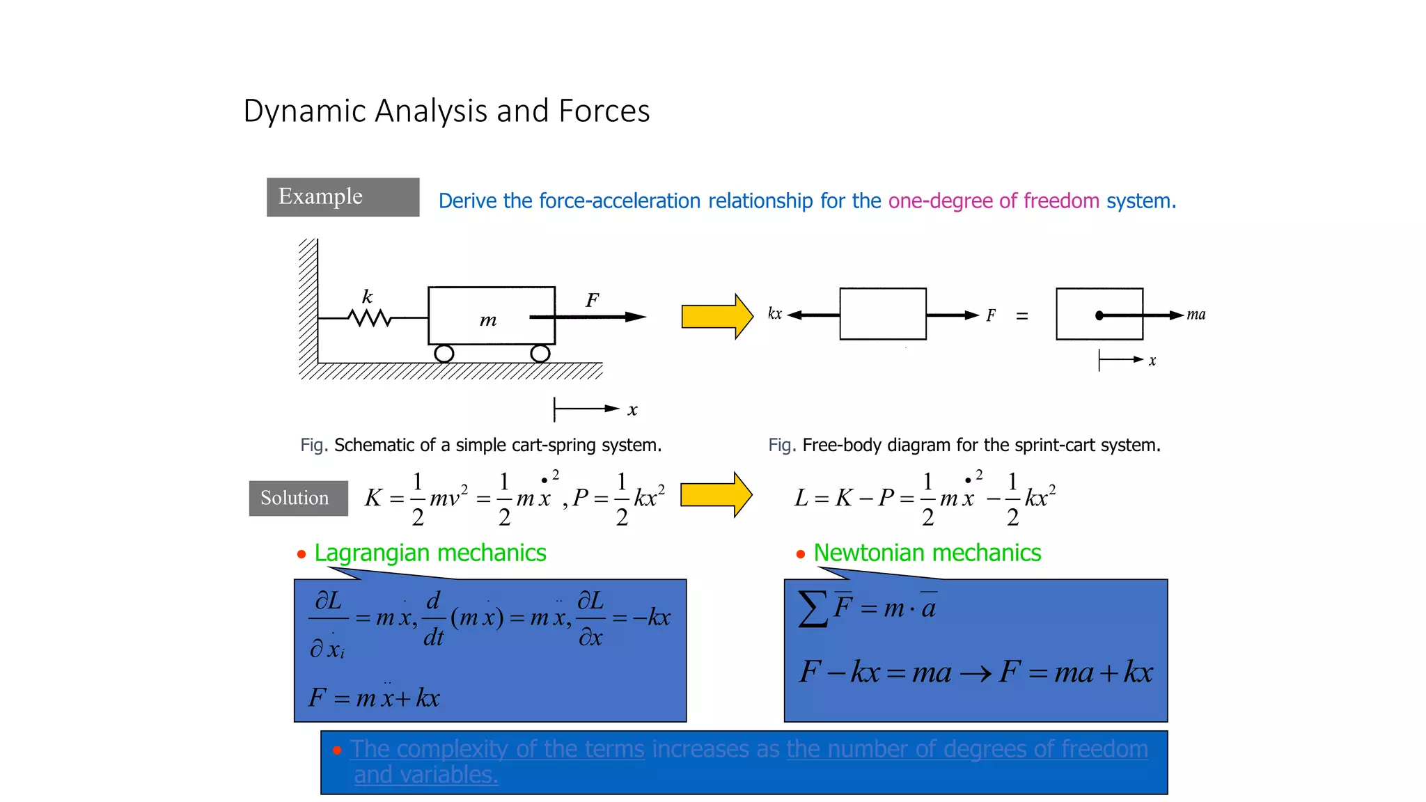
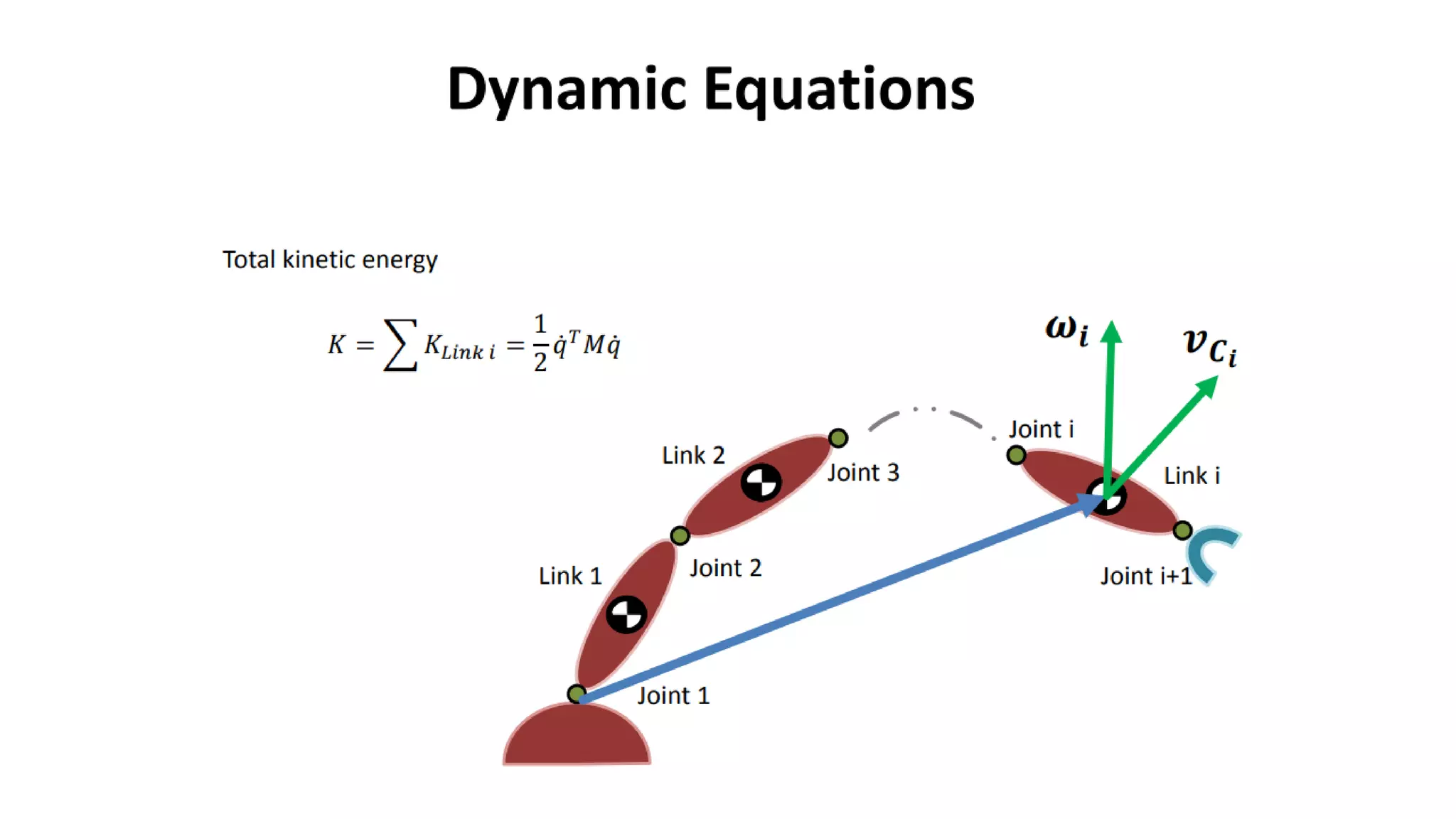
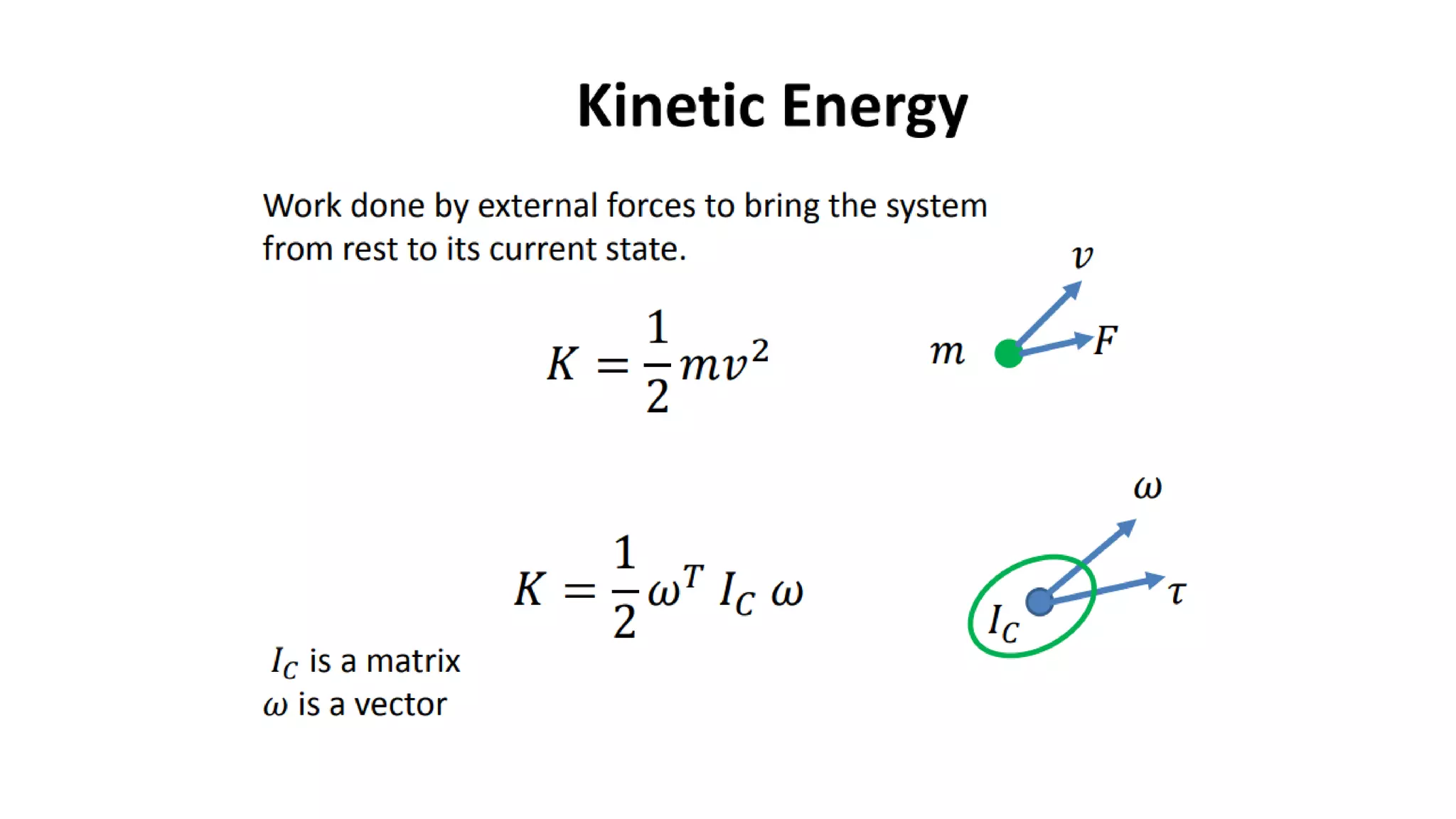
![Dynamic Analysis and Forces
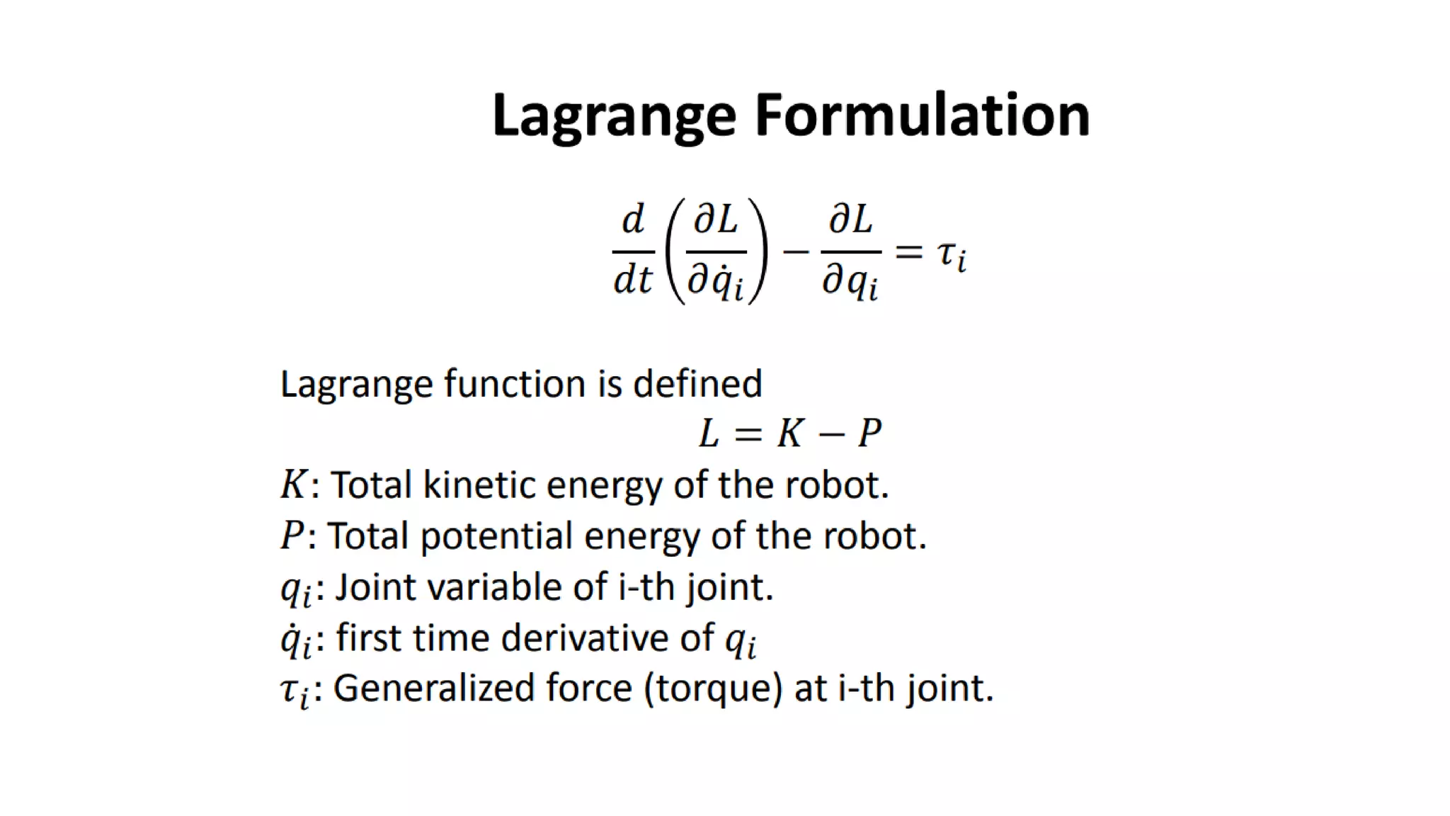
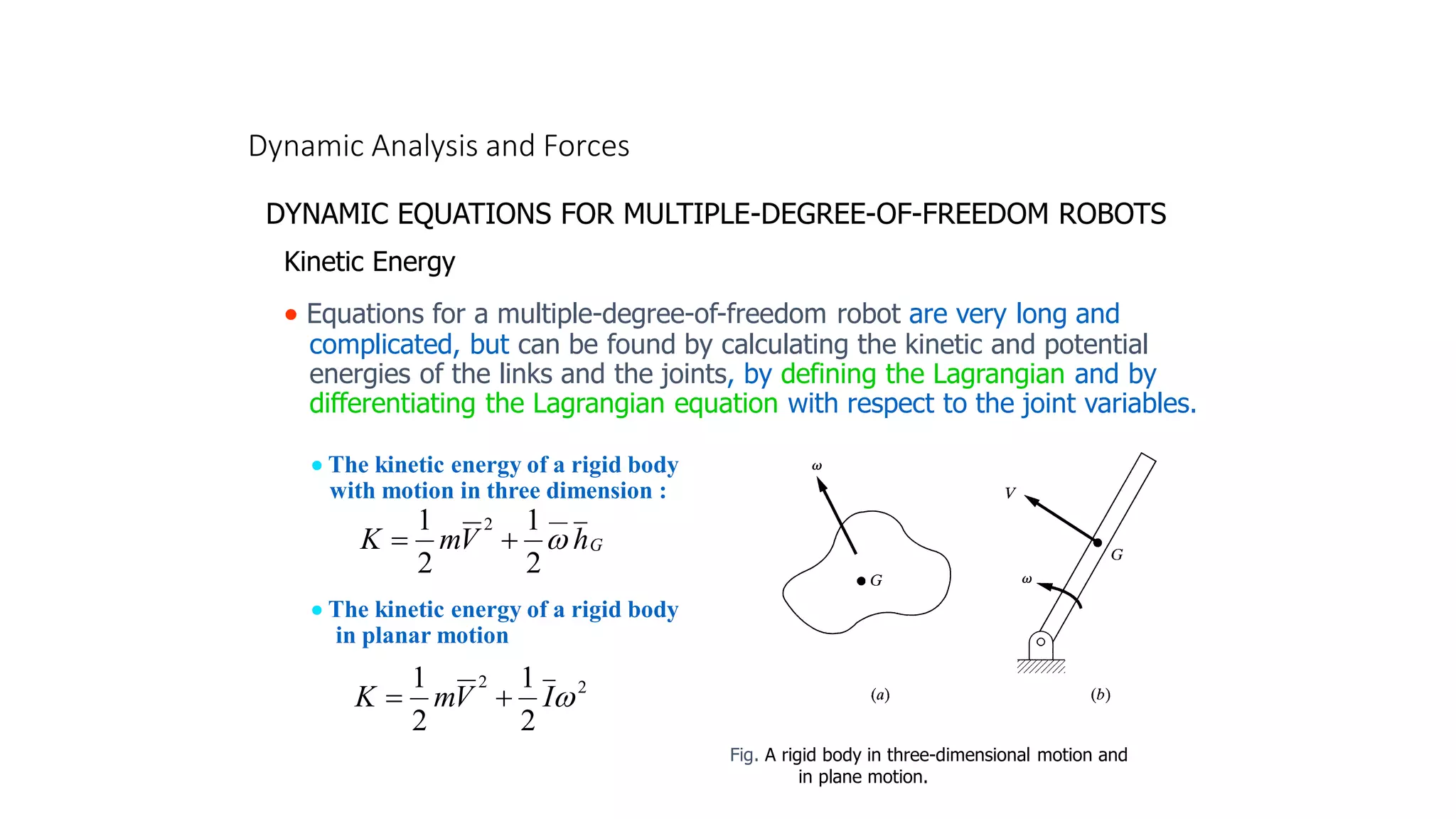
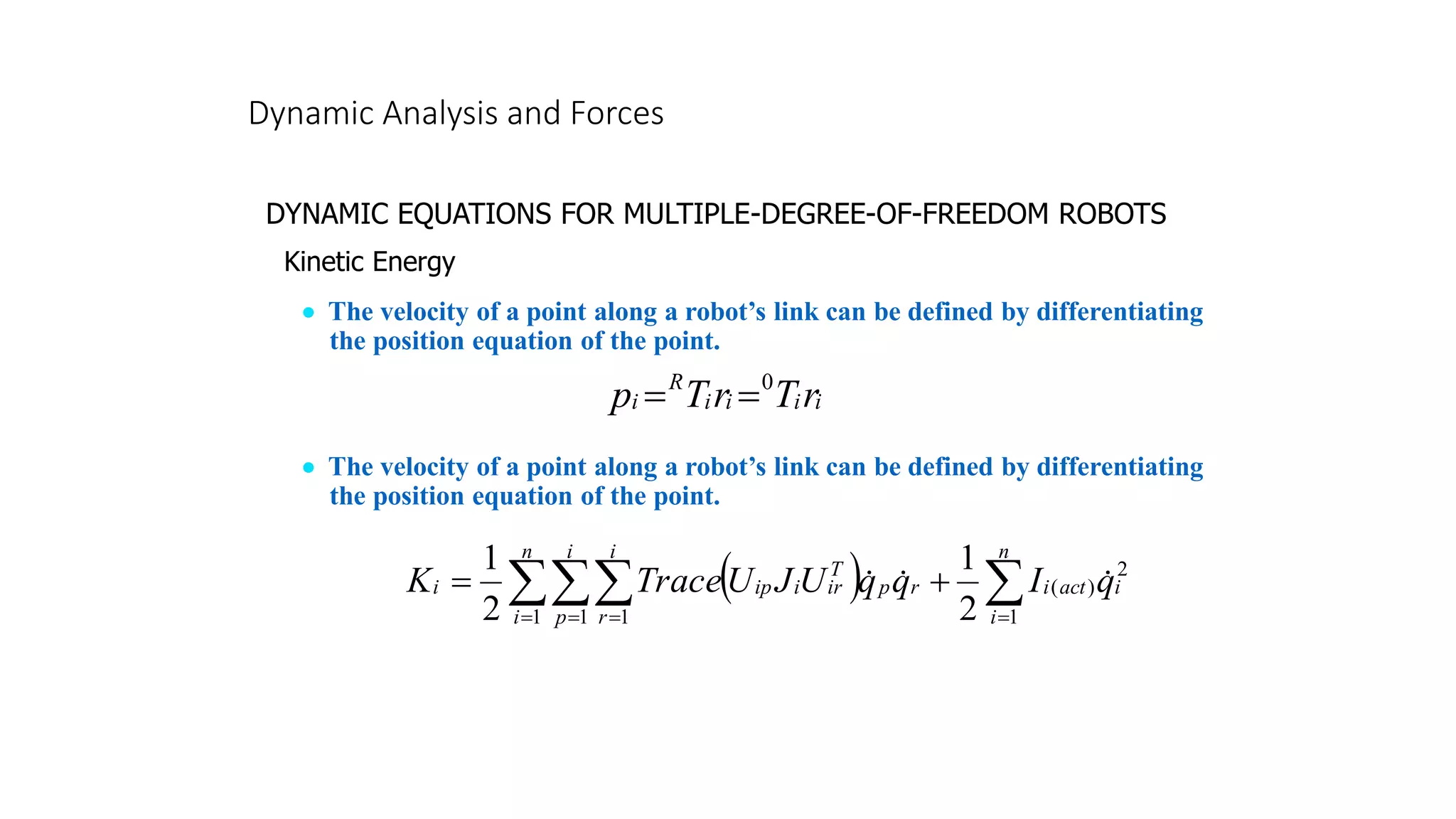
DYNAMIC EQUATIONS FOR MULTIPLE-DEGREE-OF-FREEDOM ROBOTS
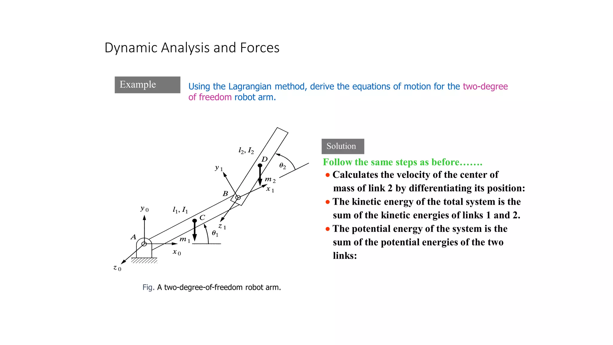
Potential Energy
• The potential energy of the system is the sum of the potential energies of each link.
]
)
(
[
1
0
1
=
=
−
=
=
n
i
i
i
T
i
n
i
i r
T
g
m
p
P
• The potential energy must be a scalar quantity and the values in the gravity
matrix are dependent on the orientation of the reference frame.](https://image.slidesharecdn.com/2-kinamaticsintroductionforwardandreversekinematicsrobotarmanddegreesoffreedom-15-05-20231-230825154206-353c20af/75/2-Kinamatics-Introduction-forward-and-reverse-kinematics-robot-arm-and-degrees-of-freedom-15-05-2023-1-pdf-94-2048.jpg)
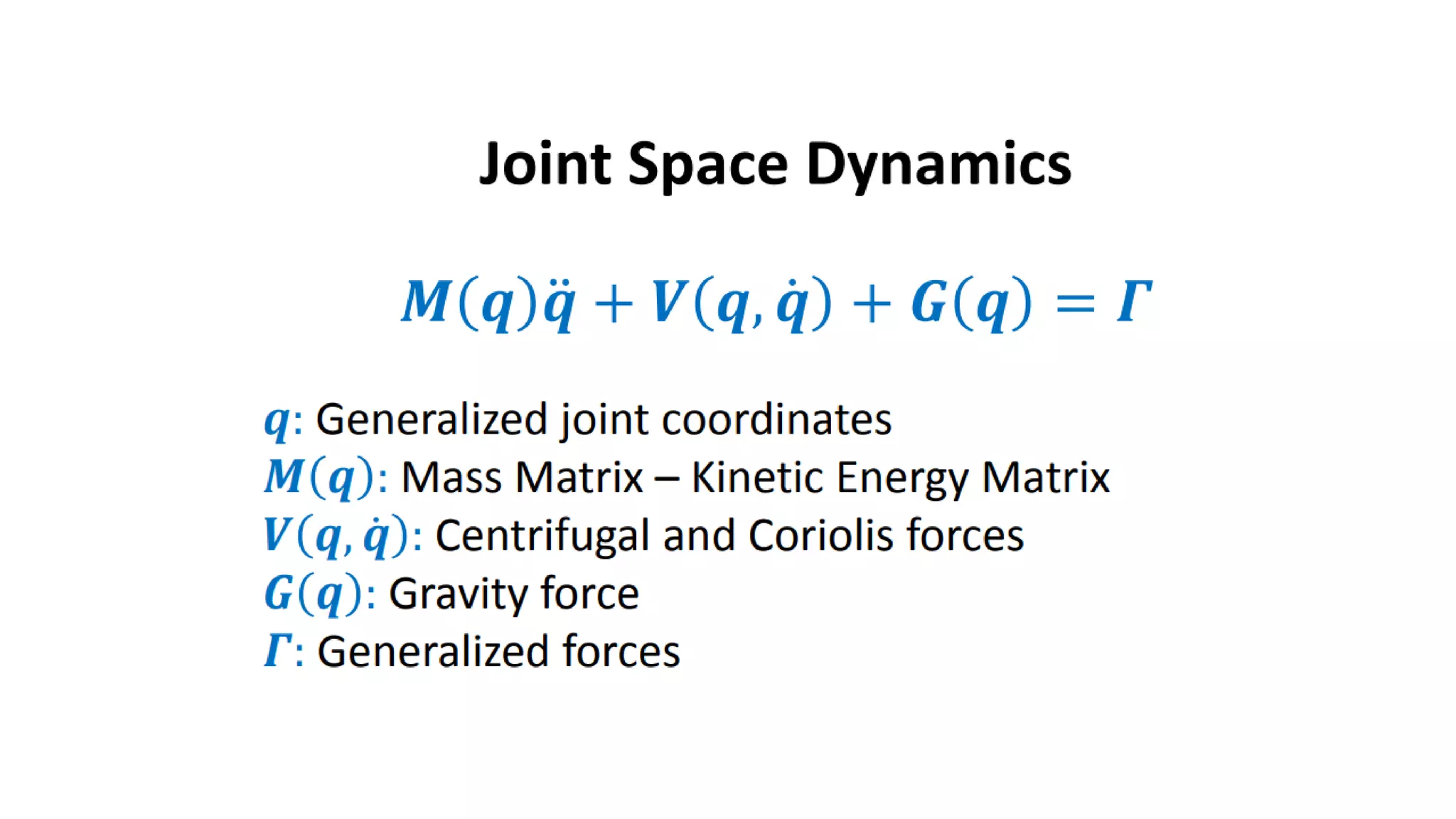
![Dynamic Analysis and Forces
DYNAMIC EQUATIONS FOR MULTIPLE-DEGREE-OF-FREEDOM ROBOTS
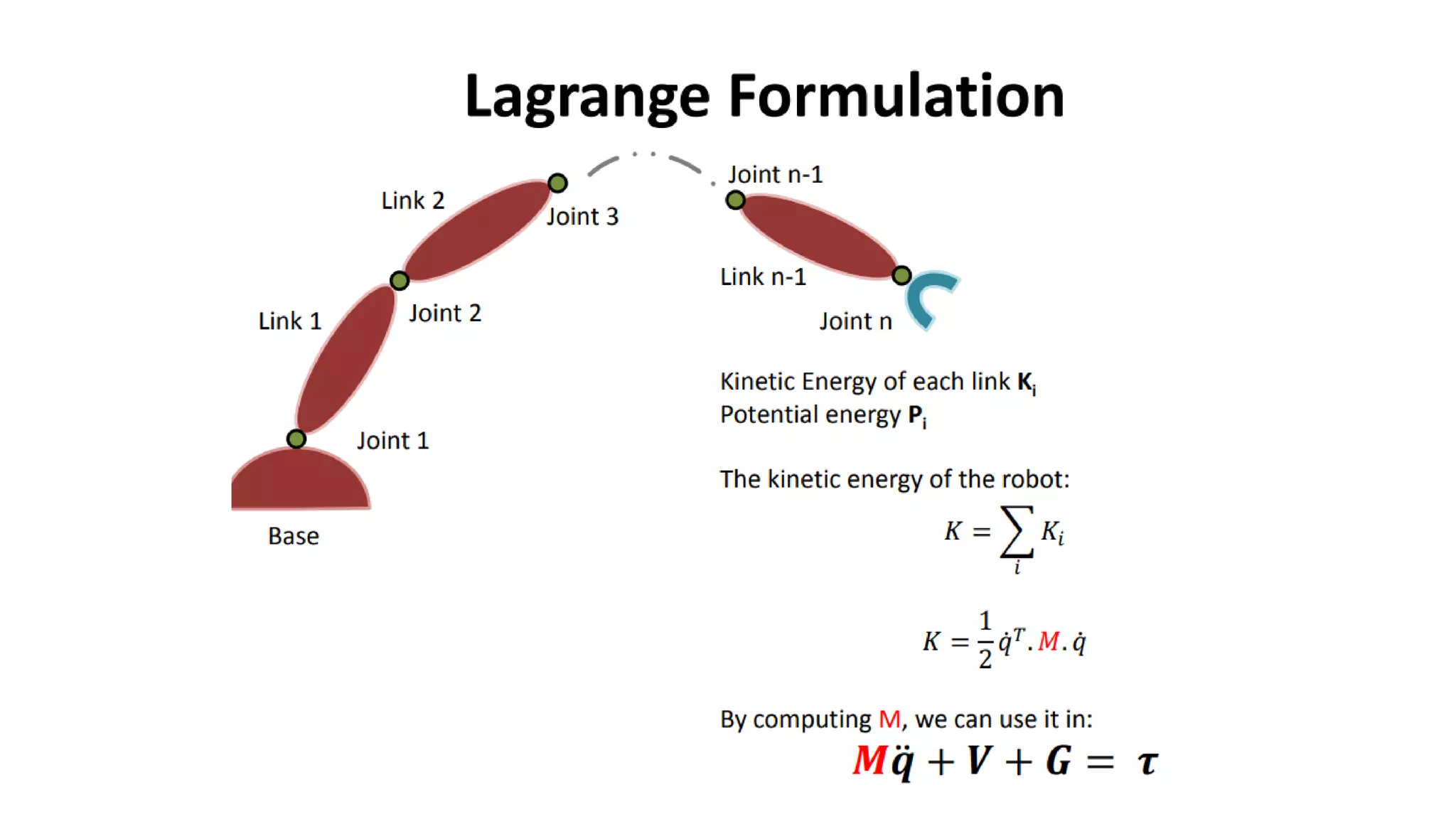
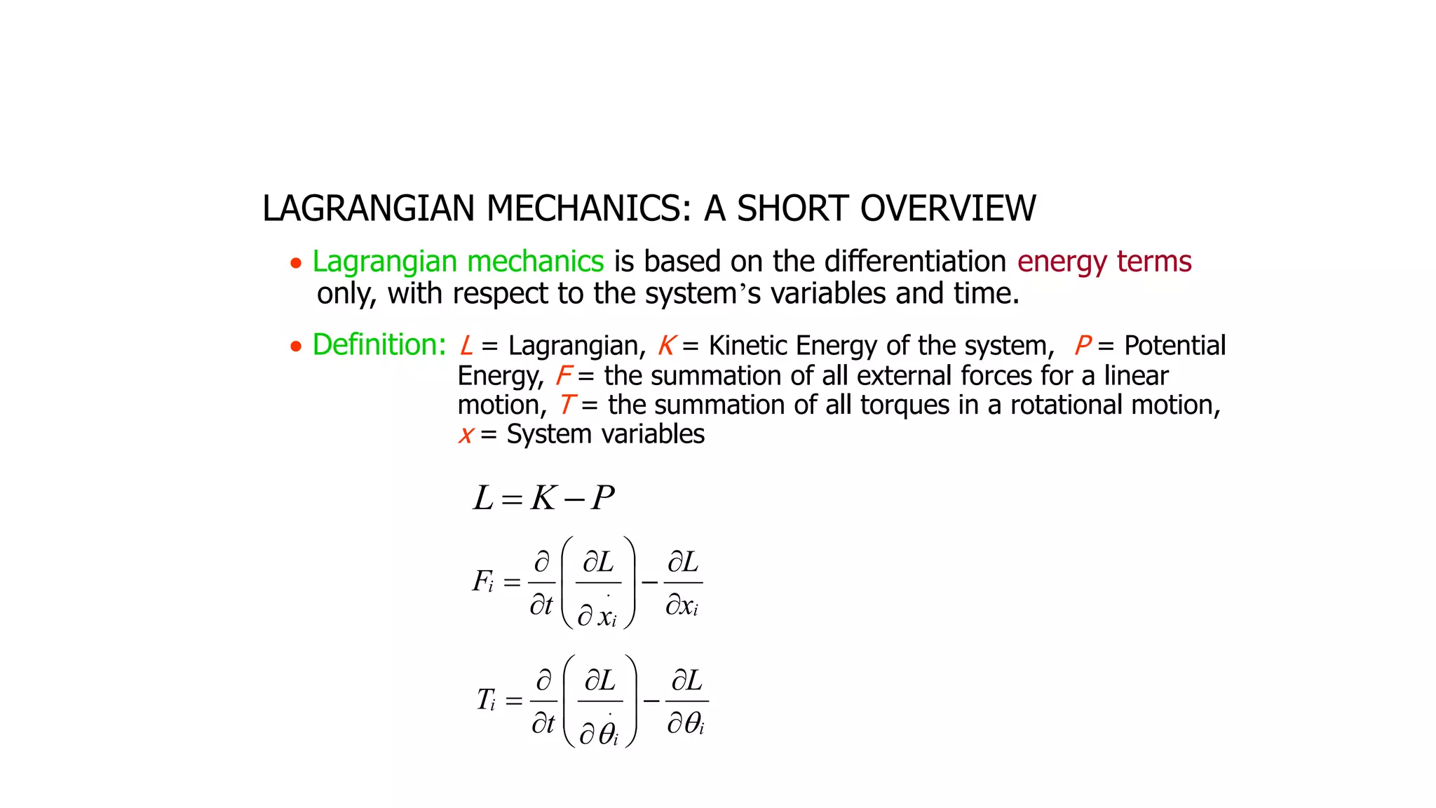
The Lagrangian
( ) r
n
i
i
p
i
r
p
T
ir
i
ip q
q
U
J
U
Trace
P
K
L
= = =
=
−
=
1 1 1
2
1
]
)
(
[
2
1
1
0
1
2
)
(
=
=
−
−
+
n
i
i
i
T
i
n
i
i
act
i r
T
g
m
q
I ](https://image.slidesharecdn.com/2-kinamaticsintroductionforwardandreversekinematicsrobotarmanddegreesoffreedom-15-05-20231-230825154206-353c20af/75/2-Kinamatics-Introduction-forward-and-reverse-kinematics-robot-arm-and-degrees-of-freedom-15-05-2023-1-pdf-95-2048.jpg)
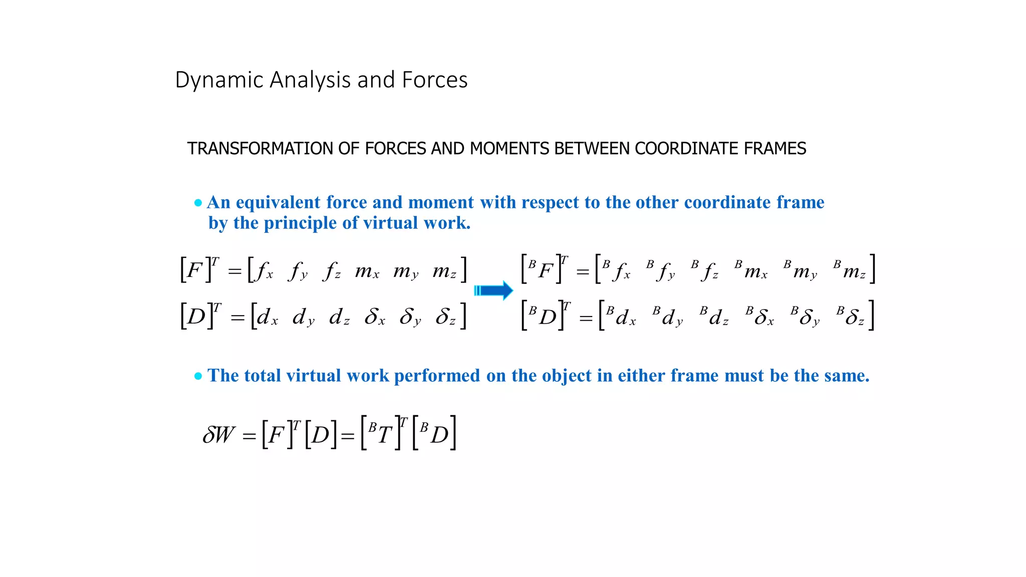
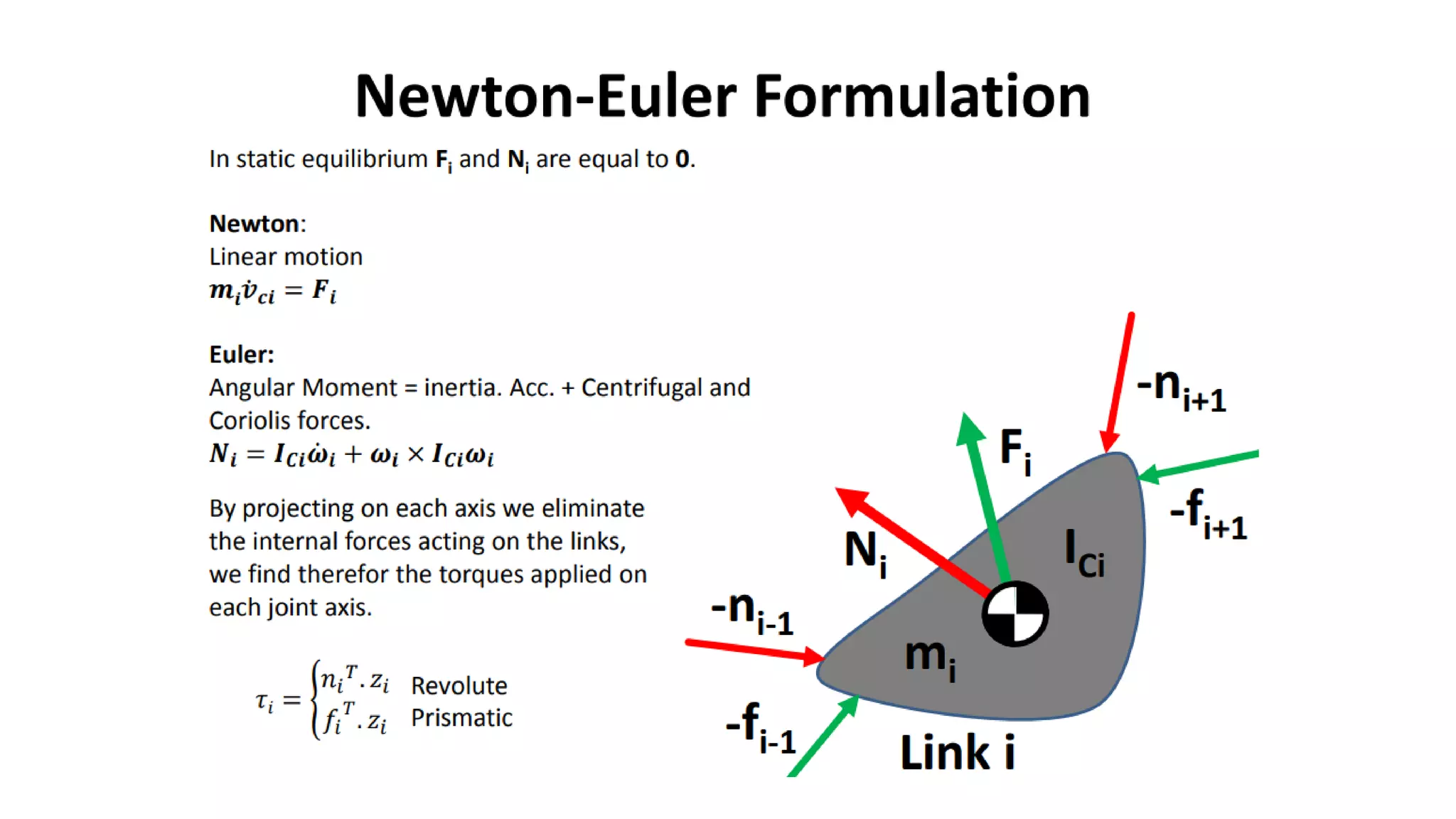
![Dynamic Analysis and Forces
TRANSFORMATION OF FORCES AND MOMENTS BETWEEN COORDINATE FRAMES
• Displacements relative to the two frames are related to each other by the
following relationship.
D
J
D B
B
=
• The forces and moments with respect to frame B is can be calculated directly
from the following equations:
f
n
fx
B
=
f
o
fy
B
=
f
o
fy
B
=
( ) ]
[ m
p
f
n
mx
B
+
=
( ) ]
[ m
p
f
o
my
B
+
=
( ) ]
[ m
p
f
a
mz
B
+
=](https://image.slidesharecdn.com/2-kinamaticsintroductionforwardandreversekinematicsrobotarmanddegreesoffreedom-15-05-20231-230825154206-353c20af/75/2-Kinamatics-Introduction-forward-and-reverse-kinematics-robot-arm-and-degrees-of-freedom-15-05-2023-1-pdf-101-2048.jpg)
![The Instantaneous Centre of Curvature [ICC]](https://image.slidesharecdn.com/2-kinamaticsintroductionforwardandreversekinematicsrobotarmanddegreesoffreedom-15-05-20231-230825154206-353c20af/75/2-Kinamatics-Introduction-forward-and-reverse-kinematics-robot-arm-and-degrees-of-freedom-15-05-2023-1-pdf-124-2048.jpg)
![The Instantaneous Centre of Curvature [ICC]
• Consider the case where several wheels are in contact
with the surface – see previous slide.
• If all wheels in contact with the surface are to roll –
then the axes of each wheel must intersect through a
single centre of rotation – the ICC (case a).
• If no consistent ICC exists then the wheels cannot roll
(case b).
• Not only must the ICC exist but each wheel’s velocity
must be consistent with a rigid rotation about the ICC.
E.g. If a set of three wheels were equidistant from the
ICC they would all have to move at the same velocity.](https://image.slidesharecdn.com/2-kinamaticsintroductionforwardandreversekinematicsrobotarmanddegreesoffreedom-15-05-20231-230825154206-353c20af/75/2-Kinamatics-Introduction-forward-and-reverse-kinematics-robot-arm-and-degrees-of-freedom-15-05-2023-1-pdf-125-2048.jpg)
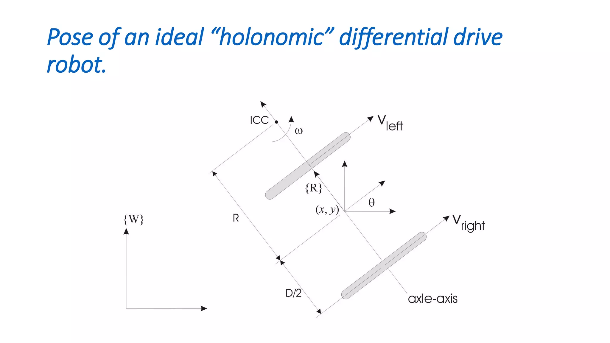
![Where is the ICC?
• So for each wheel on the robot
• [1]
• [2]
• Assuming we know VLeft and VRight (i.e. we can control the speed of the
wheels!)
• We can then solve the simultaneous equations for ω and R.
)
2
( D
R
VLeft −
=
)
2
( D
R
VRight +
= ](https://image.slidesharecdn.com/2-kinamaticsintroductionforwardandreversekinematicsrobotarmanddegreesoffreedom-15-05-20231-230825154206-353c20af/75/2-Kinamatics-Introduction-forward-and-reverse-kinematics-robot-arm-and-degrees-of-freedom-15-05-2023-1-pdf-132-2048.jpg)
![Solving for R:
• From [1] and from [2]
• So:
• Therefore:
2
D
R
VLeft
−
=
2
D
R
VRight
+
=
)
(
2
)
(
Left
Right
Right
Left
V
V
V
V
D
R
−
+
=
2
2 D
R
V
D
R
V Right
Left
+
=
−
)
2
(
)
2
( D
R
V
D
R
V Right
Left −
=
+
2
.
.
2
.
. D
V
R
V
D
V
R
V Right
Right
Left
Left −
=
+ R
V
R
V
D
V
D
V Left
Right
Right
Left .
.
2
.
2
. −
=
+
)
.(
)
(
2
Left
Right
Right
Left V
V
R
V
V
D
−
=
+](https://image.slidesharecdn.com/2-kinamaticsintroductionforwardandreversekinematicsrobotarmanddegreesoffreedom-15-05-20231-230825154206-353c20af/75/2-Kinamatics-Introduction-forward-and-reverse-kinematics-robot-arm-and-degrees-of-freedom-15-05-2023-1-pdf-133-2048.jpg)
![Solving for ω:
• From [1] from [2]
• Therefore:-
R
D
VLeft
=
+ 2
R
D
VRight
=
− 2
D
V
V Left
Right )
( −
=
2
2 D
V
D
V Right
Left
−
=
+
Right
Left V
D
V
=
+
Right
Left V
D
V =
+ .
Left
Right V
V
D −
=
.
](https://image.slidesharecdn.com/2-kinamaticsintroductionforwardandreversekinematicsrobotarmanddegreesoffreedom-15-05-20231-230825154206-353c20af/75/2-Kinamatics-Introduction-forward-and-reverse-kinematics-robot-arm-and-degrees-of-freedom-15-05-2023-1-pdf-134-2048.jpg)