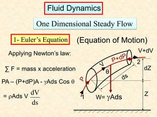
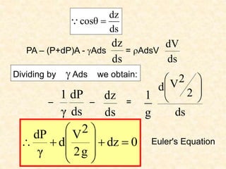
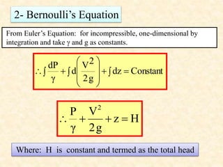
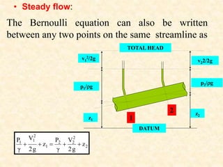
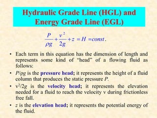
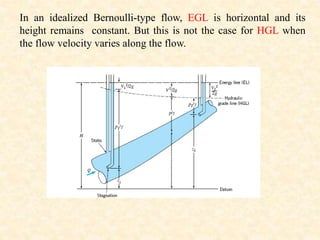
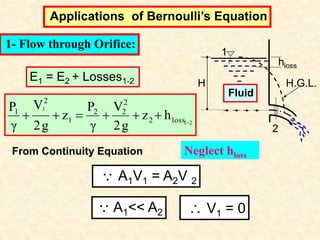
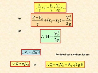
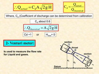
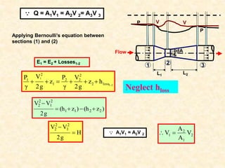
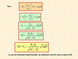
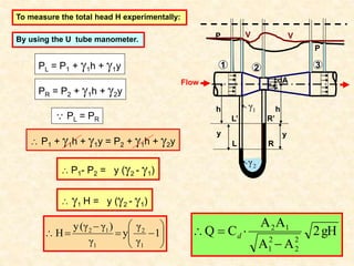
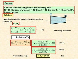
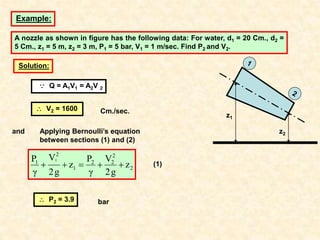
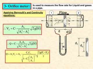
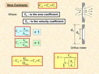
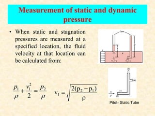
1. The document discusses the concepts of Euler's equation, Bernoulli's equation, and their applications in fluid dynamics problems involving one-dimensional steady flow. 2. Bernoulli's equation relates the total pressure, velocity, and elevation along a streamline. It is used to analyze flow through orifices, venturi meters, and orifice meters. 3. Measurement techniques like the pitot-static tube and manometers are used to experimentally determine velocities and pressure losses based on the equations.

1. One Dimensional Steady Flow
1- Euler’s Equation (Equation of Motion)
Fluid Dynamics
θ
W= Ads
V+dV
Z
dZ
1
2
Applying Newton’s law:
∑ F = mass x acceleration
PA – (P+dP)A - Ads Cos 
= Ads V
ds
dV

2. ds
dz
cosθ 

ds
dV
PA – (P+dP)A - Ads = AdsV
ds
dz
Dividing by  Ads we obtain:
– – =
ds
dz
ds
dP
γ
1
g
1
ds
2
2
V
d 







0
dz
g
2
2
V
d
γ
dP











 Euler's Equation

3. 2- Bernoulli’s Equation
From Euler’s Equation: for incompressible, one-dimensional by
integration and take  and g as constants.
Constant
dz
g
2
2
V
d
γ
dP



 










H
z
g
2
V
γ
P 2




Where: H is constant and termed as the total head

4. • Steady flow:
The Bernoulli equation can also be written
between any two points on the same streamline as
DATUM
z2
z1
p2/g
v22/2g
p1/g
v1
2/2g
2
1
TOTAL HEAD
2
2
2
2
1
2
1
1
z
g
2
V
γ
P
z
g
2
V
γ
P






5. Hydraulic Grade Line (HGL) and
Energy Grade Line (EGL)
• Each term in this equation has the dimension of length and
represents some kind of “head” of a flowing fluid as
follows:
• P/ρg is the pressure head; it represents the height of a fluid
column that produces the static pressure P.
• v2/2g is the velocity head; it represents the elevation
needed for a fluid to reach the velocity v during frictionless
free fall.
• z is the elevation head; it represents the potential energy of
the fluid.
2
.
2
P v
z H const
g g

   

6. In an idealized Bernoulli-type flow, EGL is horizontal and its
height remains constant. But this is not the case for HGL when
the flow velocity varies along the flow.

7. Static, Dynamic, and Stagnation
Pressures
• The sum of the static, dynamic, and hydrostatic
pressures is called the total pressure. Therefore,
the Bernoulli equation states that the total pressure
along a streamline is constant.
• The sum of the static and dynamic pressures is
called the stagnation pressure, and it is expressed
as
2
( )
2
stag
v
P P kPa

 

8. Measurement of static and dynamic
pressure
• When static and stagnation
pressures are measured at a
specified location, the fluid
velocity at that location can
be calculated from:


2
2
1
1
2
p
v
p





)
p
p
(
2
v 1
2
1
Pitot- Static Tube

9. Bernoulli’s equation is assumed to hold along the center
streamline
If the tube is horizontal, z1 = z2 and we can solve
for V2:
We relate the velocities from the incompressible continuity relation

10. Example(8-1)
Water is flowing from a hose attached to a water main at 400 kPa gage. A
child places his thumb to cover most of the hose outlet, increasing the
pressure upstream of his thumb, causing a thin jet of high-speed water to
emerge. If the hose is held upward, what is the maximum height that the jet
could achieve?
Solution
2 2
1
2 3 2
400 1000 / 1 . /
(1000 / )(9.81 / ) 1 1
40.8
atm
P P kPa N m kg m s
z
g kg m m s kPa N
m

  

    
  





















 2
2
2
2
1
2
1
1
2
2
gz
v
p
m
gz
v
p
m
o
o


Z1 = 0.0, v1 = 0.0, v2 = 0.0, p2 = patm

11. A piezometer and a pitot tube are tapped into a horizontal water pipe, to measure
static and stagnation (static + dynamic) pressures. For the indicated water column
heights, determine the velocity at the center of the pipe.
Example(8-2)
Solution
• P1 = ρg(h1+h2)
• P2 = ρg(h1+h2 +h3)
2 2
1 1 2 2
1 2
2 2
P v P v
z z
g g g g
 
    
2
1 2 1
2
v P P
g g



Where z1 =0.0, v2 = 0.0 and z2 =0.0
2
1 2 3 1 2
1 2 1
3
( )
2
g h h h h h
v P P
h
g g g

 
   

  
2
1 3
2 2(9,81 / )(0.12 ) 1.53 /
v gh m s m m s
  

12. Applications of Bernoulli’s Equation
1- Flow through Orifice:
Fluid
2
H
2
1
1
loss
2
2
2
2
1
2
1
h
z
g
2
V
γ
P
z
g
2
V
γ
P







E1 = E2 + Losses1-2 H.G.L.
1
hloss
 A1V1 = A2V 2
 A1<< A2  V1 = 0
From Continuity Equation Neglect hloss

13. 2
2
2
2
1
1
z
g
2
V
γ
P
z
γ
P





H
g
2
V2 

g
2
V
)
z
(z
γ
P
P 2
2
2
1
2
1




g
2
V
H
2
2


or
or
For ideal case without losses
 Q = A2V2 H
g
2
A
V
A
Q 2
2
2 


or

14. H
g
2
A
C
Q d

 actual
H
g
2
A
Q 
 l
theoretica
Where, Cd (Coefficient of discharge can be determined from calibration
Cd about 0.6
Cd =1 Hloss= 0
or
2- Venturi meter:
Is used to measure the flow rate
for Liquid and gases.
1
2
3
throat
z1
z2
z3
Datum
section
section
l
theoretica
actual
d
Q
Q
C 

15. 1 2 3
P
P V
V
Flow
 Q = A1V1 = A2V 2= A3V 3
dA
2
1
1
loss
2
2
2
2
1
2
1
h
z
g
2
V
γ
P
z
g
2
V
γ
P







)
z
(h
)
z
(h
g
2
V
V
2
2
1
1
2
1
2
2





Applying Bernoulli’s equation between
sections (1) and (2)
E1 = E2 + Losses1-2
L1
L2
H
g
2
V
V 2
1
2
2


 A1V1 = A2V 2 2
1
2
1 V
A
A
V 

Neglect hloss

16. H
g
2
A
A
1
V 2
1
2
2
2
2 










H
g
2
A
A
A
V
2
2
2
1
1
2



H
g
2
A
A
A
A
Q
2
2
2
1
1
2



gH
2
A
A
A
A
C
Q
2
2
2
1
1
2



 d
Cd can be estimated experimentally by calibration and its value is about 0.96.
H
g
2
V
A
A
V 2
2
2
1
2
2
2 










Then

17. To measure the total head H experimentally:
1 2 3
P
P V
V
Flow dA
R
L
R’
L’
y y
h h
By using the U tube manometer.
PL = P1 + 1h + 1y
1
γ
2
γ
PR = P2 + 1h + 2y
 PL = PR
 P1 + 1h + 1y = P2 + 1h + 2y
 P1- P2 = y (2 - 1)
 1 H = y (2 - 1)












 1
γ
γ
y
γ
)
γ
(γ
y
H
1
2
1
1
2 gH
2
A
A
A
A
C
Q
2
2
2
1
1
2



 d

18. Example:
A nozzle as shown in figure has the following data:
Q = 60 liter/sec. of water, d1 = 25 Cm., d2 = 15 Cm. and P1 = 1 bar. Find P2.
Neglect losses
Solution: 1
2
Applying Bernoulli’s equation between sections
(1) and (2)
2
2
2
2
1
2
1
z
g
2
V
γ
P
z
g
2
V
γ
P 1





E1 = E2
Assuming no losses
(1)
 Q = A1V1 = A2V 2
2
2
2
1
2
1
V
4
πd
V
4
πd
60 


 1.222
(0.25)
π
10
60
4
V 2
3
1 






m/sec.
398
.
3
)
15
(0.
π
10
60
4
V 2
3
2 






m/sec.
Substituting in (1)  P2 = 0.9486 bar

19. Example:
A nozzle as shown in figure has the following data: For water, d1 = 20 Cm., d2 =
5 Cm., z1 = 5 m, z2 = 3 m, P1 = 5 bar, V1 = 1 m/sec. Find P2 and V2.
Solution:
Applying Bernoulli’s equation
between sections (1) and (2)
2
2
2
2
1
2
1
z
g
2
V
γ
P
z
g
2
V
γ
P 1




 (1)
z1
z2
 P2 = 3.9 bar
and
 V2 = 1600 Cm./sec.
 Q = A1V1 = A2V 2

20. 3- Orifice meter: Is used to measure the flow rate for Liquid and gases
in a pipe.
2
d d/2
d1
do
 
H
g
2
A
A
A
C
V
2
2
2
1
1
2




 
H
g
2
A
A
A
A
C
Q
2
2
2
1
1
2




1
H
Applying Bernoulli’s and Continuity
equations:
Flow
γ
)
P
g(P
2
A
A
C
1
C
C
A
V
A
Q 2
1
2
1
2
2
c
v
c
2
2
2













21. Orifice meter
Cc : is the area coefficient.
.
theo
.
act
c
A
A
C 
Cv : is the velocity coefficient.
.
theo
.
act
v
V
V
C 
< 1
> 1
v
c
.
theo
.
act
d C
C
Q
Q
C 



4
1
o
d
d
d
1
C
C











d1
do
Vena Contracta: v
c
d C
C
C 

Where:

22. Z
y
Z1
Z2
V1
If V1 = 3 m/sec.
V2 = 10 m/sec.
z1 = ?? m.
z = 2 m.
z2 = 1 m.
y = ?? m.
Find:
2
2
2
2
1
2
1
z
g
2
V
γ
P
z
g
2
V
γ
P 1






 P1 = P2 = 0 z1 =( z + y ) m.
4- Open Channel Flow
y = 3.64 m.

and
V2

23. x
y
H
1
1
2
2
5- Notches and Weir:
g
2
V
h)
y
(x
g
2
V
y
x
2
2
2
1
















g
2
V
h
2
V
2
2
1
g
b
h
δh

24. Area of strip = b. δh
Velocity through the strip = gh
2
Discharge through the strip = δh gh
2
Integrating from h = 0 to h = H



H
0
th dh
bh
g
2
Q
2
1
B
b
2
3
H
g
2
B
3
2
Qth 




If b = B = constant

25. 2
θ
h
δh
If V- Notch
2
5
H
2
θ
tan
g
2
15
8
Qth 








