This document explores the application of He's variational iteration method (VIM) for solving Riccati matrix differential equations, which are known for their complexity in deriving analytical solutions. The paper establishes the convergence of an iterative sequence of approximate solutions to the exact solution using mathematical induction and outlines the methodological principles of VIM. Emphasis is placed on the effectiveness of the VIM compared to other numerical methods, citing its accuracy and efficiency in various applications.

1. Indonesian Journal of Electrical Engineering and Computer Science
Vol. 5, No. 3, March 2017, pp. 673 ~ 683
DOI: 10.11591/ijeecs.v5.i3.pp673-683  673
Received November 30, 2016; Revised February 3, 2017; Accepted February 21, 2017
Variational Iteration Method for Solving Riccati Matrix
Differential Equations
Khalid Hammood Al-jizani*, Noor Atinah Ahmad, Fadhel Subhi Fadhel
School of Mathematical Sciences, Universiti Sains Malaysia, 11800, Penang, Malaysia. +60164705290
*Corresponding author, e-mail: khm13_mah009@student.usm.my
Abstract
Riccati matrix differential equation has long been known to be so difficult to solve analytically
and/or numerically. In this connection, most of the recent studies are concerned with the derivation of the
necessary conditions that ensure the existence of the solution. Therefore, in this paper, He’s Variational
iteration method is used to derive the general form of the iterative approximate sequence of solutions and
then proved the convergence of the obtained sequence of approximate solutions to the exact solution. This
proof is based on using the mathematical induction to derive a general formula for the upper bound proved
to be converging to zero under certain conditions.
Keywords: Matrix Riccati differential equation, Variational iteration method, Iterative methods, He’s
iterative method, Matrix differential equations.
Copyright © 2017 Institute of Advanced Engineering and Science. All rights reserved.
1. Introduction
Mathematical modeling of real life problems, especially in control problems leads to
differential equations, integral equations, system of differential and algebraic equations. While
the solution of such obtained models may be so difficult to be evaluated analytically, therefore
numerical and approximate methods seem to be necessary to be used to evaluate the solution
of such problems.
Among the most popular and simplest accurate methods, the iterative methods is the
variational iteration method (VIM), which is proposed by Ji-Huan He in 1999 as a special
approach of the homotopy analysis method. The VIM has been shown to solve functional
equations efficiently. In related literature, this method has been referred to as a modification of
the general Lagrange multiplier method [18].
Several researchers compared the VIM with other numerical and approximate methods,
where it is shown by all that this method may give more accurate results and faster than the
other methods. In addition, in this method, the convergent to the exact solution is considered
into a count and proved in the research work [9].
The main feature of the VIM is that the solution of the problem under consideration with
linearization assumption is used as an initial approximate solution to more accurate and precise
approximate solution which is obtained through iterative.
The VIM has been used by other researchers to solve various problems such as He in
1999 used the VIM to give approximate solution for some well known non-linear problems, [11].
He in 2007 used this method to solve autonomous systems of ordinary differential equations,
[10]. In 2006 the VIM was applied for solving nonlinear integro-differential equation of functional
order by Kurulay M. [13, 17]. David K. and Hadi R. G. in 2010 studied the convergence of the
VIM for the solution of the telegraph problem, [3]. Ghorbani A. and Saberi J. proved the
convergence of the VIM of nonlinear oscillators with an illustrative example [6]. Nguyen T. et al
in 2010 propose a new method to solve Riccati matrix differential equation, which is based on
the differential Lyapunov equation to calculate numerically the solution of Riccati matrix
differential equation [19]. The metod of Nguyen T., et al., [19] is shown to be robust and
numerically efficient. While the application of the proposed method by Nguyen T. et al. had been
applied [20] to the singular perturbed linear quadratic optimal control problem, in which for this
objective, the author’s compose the full-order optimal linear –quadratic control problem into an
reduced order subproblems. A similar transformation idea can be found in the works of Glizer

2.  ISSN: 2502-4752
IJEECS Vol. 5, No. 3, March 2017 : 673 – 683
674
and Dmitriev [7, 8], in which a series of expansion method is proposed. Biazar J., et al., in 2011
studied the numerical solution of certain functional integral equations by the VIM [2]. Geng F.
used the modified VIM in 2009 to solving scalar Riccati differential equation [4]. Lu J. solved a
nonlinear system of second order boundary value problems using VIM in 2007 [16] while
Hemeda A.A. used the VIM to solve the wave partial differential equation [12]. The VIM has also
been used to solve more advance problems movable boundaries by Ghomanjani F. and
Ghaderi S. in 2012 [5].
In addition, in recent years, there is a wide occurrence of Riccati matrix differential
equation as a control model in which the analytical and theoretical results concerning this matrix
equation has been established, but still its solution seems to be difficult to be evaluated.
In the current study, the VIM will be used to solve Riccati matrix differential equation,
where the convergence of the sequence of iterated approximate solutions have been proved to
be converge to the exact solution of the problem, which is assumed to exist and be unique
depending on the results of the other researchers [15].
2. The Ricatti Equation
The study of scalar and Riccati matrix and/or differential equations has a great
importance, which dates from the early days of modern mathematical analysis, since such
equations represent one of the obtained types of nonlinear equations, especially in
mathematical physics. Also, within recent years, there is a wide occurrence of Riccati matrix
differential equations notably in variational theory and allied areas of optimal control, invariant
embedding and dynamic programming [21].
An atypical algebraic Riccati equation is similar to one of the following [14, 22]. The first
is a quadratic matrix equation for the unknown n n matrix X of the form:
0T
A X XA XBX C    (1)
Where ,A B and C are n n complex matrices with B and C hermitian, and T refers to the
matrix transpose. Equation (1) is called the continuous time Riccati equation.
The second equation has the functional form for the unknown n n matrix X .
1
( ) ( ) ( )T T T T T
X A XA C B XA R B XB C B XA Q
      (2)
Where R and Q are m m and n n matrices respectively and , ,A B C are complex matrices
with respect to sizes n n , n m and m n respectively. In addition, both equations arise in
systems theory, differential equations and filter design in control theory [14].
More advanced and interesting form of Riccati matrix equation is the nonlinear Riccati
matrix differential equation of the form [21]:
0T
X XA A X XBX C     (3)
Where ,A B and C are constants n n matrices such that T
B B and T
C C . The existence
conditions of a unique solution are imposed and satisfied on equation (3).
Solution of equation (3) may be achieved analytically, which is so complicated and
difficult to evaluate in some cases and therefore numerical and/or approximate methods seems
to be necessary to find the solution of equation (3). In the next section, we will present and use
one of the He’s iteration methods to solve equation (3), namely we will use the VIM.
3. The Variational Iteration Method
To illustrate the basic ideas of the VIM, consider the following nonlinear equation given
in abstract form as an operator equation:
( ) ( )Au t g t , t  [a, b] (4)

3. IJEECS ISSN: 2502-4752 
Variational Iteration Method for Solving Riccati Matrix Differential… (Khalid Hammood Al-jizani)
675
Where Ais a nonlinear operator, ( )g t is a given function, ,a b and u is the unknown
function. If it is assumed that the operator A may be decomposed into two operators, namely; L
and N that will be rewritten equation (4) as follows:
( ) ( ) ( )Lu t Nu t g t  (5)
Where L is a linear operator, N is a nonlinear operator and g is any given function, which is
called the nonhomogeneous term.
The analysis of the VIM is to rewrite equation (5) as follows:
( ) ( ) ( ) 0Lu t Nu t g t   (6)
And if it is supposed that un is the
th
n approximate solution of equation (6), then it follows that:
( ) ( ) ( ) 0n nLu t Nu t g t   (7)
And therefore, a correction functional for equation (5) may be given by:
 
0
1( ) ( ) ( ) ( ) ( ) ( )
t
n n n n
t
u t u t s Lu s Nu s g s ds      (8)
Where  is the general Lagrange multiplier that can be identified optimally via variational theory,
the subscript n denotes the
th
n iterative approximate solution of u, and nu is considered as a
restricted variation, i.e., 0nu  , [1].
To solve equation (8) by the VIM, the Lagrange multiplier  should be determined and
evaluated first that will be identified optimally through integration by parts. Then, the successive
approximations ( )nu t , n  0, 1, …; of the solution u(t) was obtained upon applying the obtained
Lagrange multiplier .
Now, using selective function 0( )u t as an initial guess for ( )u t , the zero
th
approximation 0u may be selected by any function that just satisfies at least the initial and
boundary conditions with  predetermined, then several approximations ( )nu t , n  0, 1, …;
follows immediately and consequently the exact solution may be arrived since:
( ) lim ( )n
n
u t u t

 (9)
In other words, the correction functional for equation (8) will give a sequence iterated
approximations, and therefore the exact solution is obtained as the limit of the resulting
successive approximations [25].
4. Approximate Solution of Riccati Matrix Differential Equations Using VIM
It is obvious now that the main aspects of the VIM requires first the determinative of the
Lagrange multiplier ( )t , which may be found by the method of integration by parts, i.e. , for
equation (8) that can be used:
0 0
( ) ( ) ( ) ( ) ( ) ( )
t t
n n n
t t
t u t dt t u t t u t dt      

4.  ISSN: 2502-4752
IJEECS Vol. 5, No. 3, March 2017 : 673 – 683
676
0 0
( ) ( ) ( ) ( ) ( ) ( ) ( ) ( )
t t
n n n n
t t
t u t dt t u t t u t t u t dt         
And so on. Therefore, after having determined ( )t , the sequence of approximate solutions
, 0,1,...1 nnu  ,
of the solution will be obtained immediately upon any selective function u as an
initial guess. As it is found previously in literatures (see for example [23,24]), the general form of
( )t for the
th
n order ODE:
( ) ( 1)( ) ( , ( ), ( ),..., ( )) 0n nu t f t u t u t u t  (10)
Is proved by induction to be:
11
( ) ( 1) ( )
( 1)!
n n
t t x
n
 
  

(11)
Where it is clear that for the first order ODE ( ) 1t   , for the second order ODE ( ) 1t  
and so on.
The generalization of the correction functional (8) with its corresponding Lagrange
multiplier for systems of n-operator equations may be considered similarly by using system of n-
correction functionals with related n-Lagrange multiplier.
Hence, in connection with Ricaati matrix differential equation (3), the correction
functional may be considered for a system of n-equations of the first order ODE’s as follows:
Equation (3) may be written in the form of equation (10) as:
( ) ( , ( ) 0X t F t X t  (12)
Where,
( , ( )) ( ) ( ) ( ) ( )T
F t X t AX t X t A X t BX t C   
And hence equation (3) (or equivalently equation 12) may be written in the form of the nonlinear
equation (4), where the related nonlinear operator in the lefthand side of equation (4) is defined
by:
Td
A A A B
dt
     (13)
And the nonhomogenuous function in the righthand side is given by:
( )  g t C (14)
Therefore, in connection with the nonlinear operator (13) that may be decomposed into two
operators, namely; a linear operator L and a nonlinear operator N , which are defined as:
Td
L A A
dt
    (15)
N B    (16)

5. IJEECS ISSN: 2502-4752 
Variational Iteration Method for Solving Riccati Matrix Differential… (Khalid Hammood Al-jizani)
677
Hence, the statement of the variational iteration formula (8) related to the Riccati matrix
differential equation:
( ) ( ) ( )LX t NX t g t  (17)
Where L, N and g are defined by equations (14), (15) and (16) respectively. The derivation of
the approximated formula is presented and it is easily verified that the correction functional
takes the form as in the next theorem.
Theorem (1):
The correction functional of the Ricaati matrix differential equation (3) has the form:
0
1( ) ( ) [ ( ) ( ) ( ) ( ) ( ) ]
t
T
n n n n n n
t
X t X t X s X s A A X s X s BX s C ds       (18)
For all n=0,1,…
Proof:
Rewrite equation (3) in the form of equation (12) in matrix form. Then using the resulting
Lagrange multiplier for equations (10) and (11) implies that the nxn values of the Lagrange
multiplier ( )t to be ( ) 1.t  
In order to ensure the convergence of the sequence of approximate solutions obtained
by using equation (18), which may be proved to be converge to the exact solution ( )X s . Before
introducing the proof, the nonlinear operator M is defined by:
MX XBX
Which is assumed to satisfy Lipschitz condition with constant L, i.e., satisfy:
1 1 2 2 1 2  X BX X BX L X X (19)
Where || || is an appropriate matrix norm.
Theorem (2):
Let
1
1,..., ( [0, ],|| || )nX X C b   , n  0,1,…; be the exact and approximate solutions of
the Riccati matrix differential equation (1). If ( ) ( ) ( ) n nE t X t X t and  MX XBX satisfies
Lipschitz condition with constant L, then the sequence of approximate solutions  ( )nX t , n 
0,1,…; converges to the exact solution ( )X t .
Proof
The approximate solution of Riccati matrix equation (1) using the VIM is given by (18)
and since X is the exact solution, then it satisfy:
0
[ ]
t
T
t
X X X XA A X XBX C ds      (20)
Now, substract equation (20) from equation (18) to get:
0
1 [ ]
t
T T
n n n n n n n
t
X X X X X X A X A X BX C X XA XA XBX C ds             

6.  ISSN: 2502-4752
IJEECS Vol. 5, No. 3, March 2017 : 673 – 683
678
Since n nE X X  , then:
0
1( ) ( ) [ ( ) ( ) ( ) ( ( ) ( ) ( ) ( ))]
t
T
n n n n n n n
t
E t E t E s E s A A E s X s BX s X s BX s ds      
0 0 0 0
( ) ( ) ( ) ( ) ( ( ) ( ) ( ) ( ))
t t t t
T
n n n n n n
t t t t
E t E s ds E s Ads A E s ds X s BX s X s BX s ds         (21)
And upon using the method of integration by parts for the first integral of equation (21), to get:
0 0
1( ) ( ) ( ) (0) ( ) ( )
t t
T
n n n n n n
t t
E t E t E t E E s Ads A E s ds       
0
( ( ) ( ) ( ) ( ))]
t
n n
t
X s BX s X s BX s ds (22)
Hence taking the suprumum norm to the both sides of equation (22) yields to:
0 0 0
1( ) ( ) ( ) ( ) ( ) ( ) ( )
t t t
T
n n n n n
t t t
E t E s A ds A E s ds X s BX s X s BX s ds      
0 0 0
( ) ( ) ( )
t t t
T
n n n
t t t
E s A ds A E s ds L E s ds    
0
(2 ) ( )
t
n
t
A L E s ds  
Therefore:
0
1( ) (2 ) ( )
t
n n
t
E t A L E s ds   
Now, if n=0, then:
0
1 0( ) (2 ) ( )
t
t
E t A L E s ds  
0
0
0
[ , ]
(2 ) sup ( )
t
s t b
t
A L E s ds

  
0
0
[ , ]
(2 ) sup ( )
s t b
A L t E s

 
If n=1, then:
0
2 1( ) (2 ) ( )
t
t
E t A L E s ds  

7. IJEECS ISSN: 2502-4752 
Variational Iteration Method for Solving Riccati Matrix Differential… (Khalid Hammood Al-jizani)
679
0
0
0
[ , ]
(2 ) [2 ) sup ( ) ]
t
s t b
t
A L A L s E s ds

  
0
0
2
0
[ , ]
(2 ) sup ( )
t
s t b
t
A L E s sds

  
0
2
2
0
[ , ]
(2 )
sup ( )
2 s t b
A L
t E s



If n=2, then:
0
3 2( ) (2 ) ( )
t
t
E t A L E s ds  
0
0
2
2
0
[ , ]
(2 )
(2 ) sup ( )
2
t
t
s t b
A L
A L s E s ds


 

0
3 3
0
[ , ]
(2 )
sup ( )
3! s t b
A L t
E s



And so on in general for any natural number n.
0
0
[ , ]
(2 )
( ) sup ( )
!
n n
n
s t b
A L t
E s E s
n 


0[ , ]
(2 )
sup ( )
!
n n
n
s t b
A L b
E s
n 


Since (2 ) 1A L b is a constant and as n then
1
0
!n
 which implies
( ) 0n
E t  as n , i.e., ( ) ( )nX t X s as n , which means that the sequence of
approximate solutions using the variational iteration formula equation (18) converge to the exact
solution of Riccati matrix differential equation .
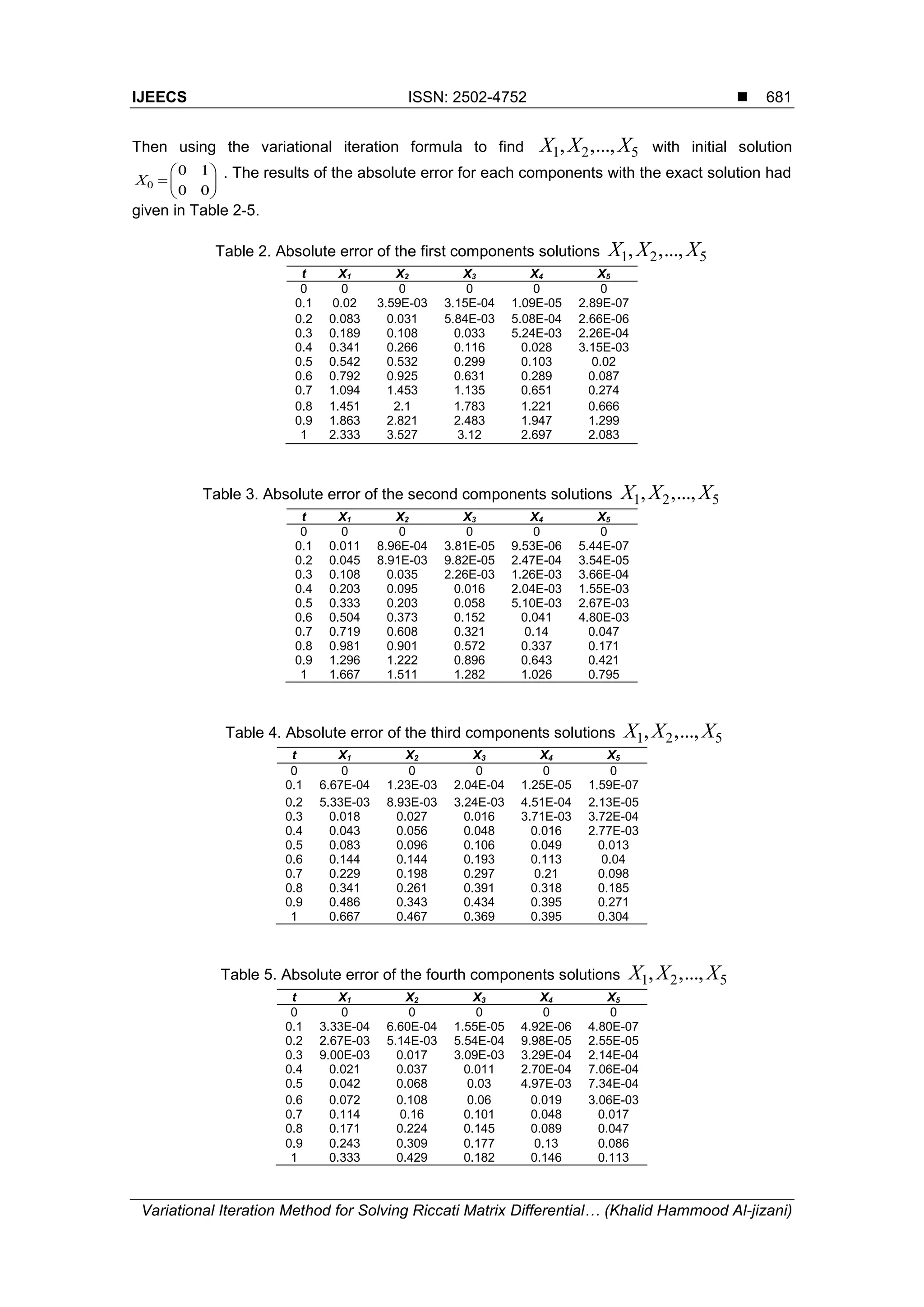
5. Illustrative Examples
In this section, two illustrative examples will be considered, where it is notable that the
matrix C may be considered as a matrix function of t which has no effect on the derivation of
the Lagrange multipliers ( )t (see theorem (1)). The first example is for the one-dimensional
Riccati differential equation while the second example is for 2 2 matrix Riccati differential
equation. In each example a comparison have been made with the exact solution.
Example (1): Consider the first order Riccati differential equation:
2 2
( ) 1 ,y x x y    [0,1]x
With initial condition (0) 1y  , where comparison with equation (3), give:
0, 1A B   and
2
1C x  

8.  ISSN: 2502-4752
IJEECS Vol. 5, No. 3, March 2017 : 673 – 683
680
The exact solution for comparison purpose is given by:
2
2
0
( )
1
x
t
t
t
e
y x x
e dt


 
 
Hence, starting with the initial solution 0( ) 1y x  , and by applying the variational
iteration formula (18), we get the first three approximate solutions:
0
2 2
1 0 0 0( ) ( ) [ ( ) 1 ( )]
t
t
y x y x y x s y s ds    
3
1
3
x
 
0
2 2
2 1 1 1( ) ( ) [ ( ) 1 ( )]
t
t
y x y x y x s y s ds    
3 4 3
(2 21)
1
3 126
x x x 
  
0
2 2
3 2 2 2( ) ( ) [ ( ) 1 ( )]
t
t
y x y x y x s y s ds    
3 5 10 7 6 4 3 4 3
(88 2310 5040 16170 93555 349272) (2 21)
1
3 5239080 126
x x x x x x x x x     
   
Also, numerical results and its comparison with the exact solution are given in Table 1.
Table 1. Absolute error between the exact and approximate solutions of example (1)
x |y1(x)  y(x)| |y2(x)  y(x)| |y3(x)  y(x)|
0 0 0 0
0.1 1.60E-05 6.45E-07 0
0.2 2.47E-04 2.00E-05 0
0.3 1.21E-03 1.48E-04 0
0.4 3.68E-03 6.10E-04 0
0.5 8.71E-03 1.83E-03 0
0.6 0.018 4.51E-03 0.001
0.7 0.032 9.72E-03 0.002
0.8 0.053 0.019 0.006
0.9 0.082 0.035 0.011
1 0.123 0.06 0.022
Example (2): Consider the 2 2 Riccati matrix differential equation with:
1 2
2 1
A
 
  
,
1 2
2 1
B
 
 
 
,
2 2
2 3
4 1 2 2 2
( )
2 3
t t t t
C t
t t
    
 
  
Which has the exact solution:
1
( )
0
t
X t
t
 
 
 

9. IJEECS ISSN: 2502-4752 
Variational Iteration Method for Solving Riccati Matrix Differential… (Khalid Hammood Al-jizani)
681
Then using the variational iteration formula to find 1 2 5, ,...,X X X with initial solution
0
0 1
0 0
X
 
  
 
. The results of the absolute error for each components with the exact solution had
given in Table 2-5.
Table 2. Absolute error of the first components solutions 1 2 5, ,...,X X X
t X1 X2 X3 X4 X5
0 0 0 0 0 0
0.1 0.02 3.59E-03 3.15E-04 1.09E-05 2.89E-07
0.2 0.083 0.031 5.84E-03 5.08E-04 2.66E-06
0.3 0.189 0.108 0.033 5.24E-03 2.26E-04
0.4 0.341 0.266 0.116 0.028 3.15E-03
0.5 0.542 0.532 0.299 0.103 0.02
0.6 0.792 0.925 0.631 0.289 0.087
0.7 1.094 1.453 1.135 0.651 0.274
0.8 1.451 2.1 1.783 1.221 0.666
0.9 1.863 2.821 2.483 1.947 1.299
1 2.333 3.527 3.12 2.697 2.083
Table 3. Absolute error of the second components solutions 1 2 5, ,...,X X X
t X1 X2 X3 X4 X5
0 0 0 0 0 0
0.1 0.011 8.96E-04 3.81E-05 9.53E-06 5.44E-07
0.2 0.045 8.91E-03 9.82E-05 2.47E-04 3.54E-05
0.3 0.108 0.035 2.26E-03 1.26E-03 3.66E-04
0.4 0.203 0.095 0.016 2.04E-03 1.55E-03
0.5 0.333 0.203 0.058 5.10E-03 2.67E-03
0.6 0.504 0.373 0.152 0.041 4.80E-03
0.7 0.719 0.608 0.321 0.14 0.047
0.8 0.981 0.901 0.572 0.337 0.171
0.9 1.296 1.222 0.896 0.643 0.421
1 1.667 1.511 1.282 1.026 0.795
Table 4. Absolute error of the third components solutions 1 2 5, ,...,X X X
t X1 X2 X3 X4 X5
0 0 0 0 0 0
0.1 6.67E-04 1.23E-03 2.04E-04 1.25E-05 1.59E-07
0.2 5.33E-03 8.93E-03 3.24E-03 4.51E-04 2.13E-05
0.3 0.018 0.027 0.016 3.71E-03 3.72E-04
0.4 0.043 0.056 0.048 0.016 2.77E-03
0.5 0.083 0.096 0.106 0.049 0.013
0.6 0.144 0.144 0.193 0.113 0.04
0.7 0.229 0.198 0.297 0.21 0.098
0.8 0.341 0.261 0.391 0.318 0.185
0.9 0.486 0.343 0.434 0.395 0.271
1 0.667 0.467 0.369 0.395 0.304
Table 5. Absolute error of the fourth components solutions 1 2 5, ,...,X X X
t X1 X2 X3 X4 X5
0 0 0 0 0 0
0.1 3.33E-04 6.60E-04 1.55E-05 4.92E-06 4.80E-07
0.2 2.67E-03 5.14E-03 5.54E-04 9.98E-05 2.55E-05
0.3 9.00E-03 0.017 3.09E-03 3.29E-04 2.14E-04
0.4 0.021 0.037 0.011 2.70E-04 7.06E-04
0.5 0.042 0.068 0.03 4.97E-03 7.34E-04
0.6 0.072 0.108 0.06 0.019 3.06E-03
0.7 0.114 0.16 0.101 0.048 0.017
0.8 0.171 0.224 0.145 0.089 0.047
0.9 0.243 0.309 0.177 0.13 0.086
1 0.333 0.429 0.182 0.146 0.113

10.  ISSN: 2502-4752
IJEECS Vol. 5, No. 3, March 2017 : 673 – 683
682
6. Conclusion
In the current study, we have applied He’s VIM to solve Riccati matrix differential
equation, which is a powerful tool that has the ability to solve different types of linear and
nonlinear operator equations. The general form of the approximate solution has been derived
depending on the general criteria of the VIM for solving n-th order ODE’s. Also, the convergence
of the obtained approximate solution have also been proved by proving the convergence of the
error term between the approximate and exact solutions to be tend to zero as the sequence of
iterations increased. The obtained results of the illustrative examples seem to be reliable in
which the absolute error between the approximate solution and the exact solution has been
used also to check the accuracy of the obtained results.
In addition, different approach based on the theory of matrix algebra may be used to
derive the approximate solution however with different rate of convergence to the exact solution
and with more restrictions on the matrices ,A Band C of the Riccati matrix differential equation,
where the approximate solution in this case has the form as follows:
0
( ) ( )
1( ) ( ) [ ( ) ( ) ( ) ( ) ( ) ]
T T
t
A A t A A s T
n n n
t
X t X t e e X s X s A A X s X s BX s C ds  
      
n=0,1.
Acknowledgements
This work is supported by the Fundamental Research Grant Scheme (FRGS) under the
MInistry of Higher Education, Malaysia.
References
[1] Batiha B, Noorani MS, Hashim I. Numerical Solutions of The Nonlinear Integro-Differential Equations.
Journal of Open Problems Compt. Math. 2008; 1(1): 34-41.
[2] Biazar J, Porshokouhi MG, Ghanbari B. Numerical solution of functional integral equations by the
variational iteration method. Journal of computational and applied mathematics. 2011; 235: 2581-
2585.
[3] Davod KS, Hadi RG. Convergence of the variational iteration method for the telegraph equation with
integral conditions. Wiley Inter Science. 2010; 27: 1442-1455,
[4] Geng F, Lin Y, Cui M. A piecewise variational iteration method for Riccati differential equations.
Computers and Mathematics with Applications. 2009; 58: 2518-2522.
[5] Ghomanjani F, Ghaderi S. Variational Iterative Method Applied to Variational Problems with Moving
Boundaries. Applied Mathematics. 2012; 3: 395-402.
[6] Ghorbani A, Saberi-Nadjafi J. Convergence of He’s variational iteration method for nonlinear
oscillators. Nonlinear Sci. Lett. A. 2010; 1(4): 379-384.
[7] Glizer VY, Dmitriev MG. Solving perturbations in a linear optimal control problem with quadratic
functional. Soviet Mathematics Doklady. 1975; 16: 1555-1558.
[8] Glizer VY, Dmitriev MG. A symptotic properties of solution of singularly perturbed Cauchy problem
encountered in optimal – control theory. Differ. Equation. 1978; 14(4): 423-432.
[9] He JH. The Variational Iteration Method: Reliable, Efficient, and Promising. An International Journal,
Computers and Mathematics with Applications. 2007; 54: 879-880.
[10] He JH, Variational Iteration Method; Some Recent Results and New Interpretations. Journal of
Computational and Applied Mathematics. 2007; 207: 3-17.
[11] He JH. Variational Iteration Method; A Kind of Non-Linear Analytical Technique; Some Examples.
International Journal of Non-Linear Mechanics. 1999; 34: 699-708.
[12] Hemeda AA. Variational iteration method for solving wave equation. Computers and Mathematics
with Applications. 2008; 56: 1948-1953.
[13] Kurulay M, Secer A. Variational Iteration Method for Solving Nonlinear Fractional Integro-Differential
Equations. International Journal of Computer Science and Emerging Technologies. 2011; 2: 18-20.
[14] Lancaster P, Rodman L. Solutions of the Continuous and Discrete Time Algebraic Riccati Equations:
A Review. In: Sergio B, Alan L, lan CW. Editors. The Riccati Equation. Springer-Verlag; 1991.
[15] Lin MN. Existence Condition on Solutions to the Algebraic Riccati Equation. Acta Automatica SINICA.
2008; 34(1).

11. IJEECS ISSN: 2502-4752 
Variational Iteration Method for Solving Riccati Matrix Differential… (Khalid Hammood Al-jizani)
683
[16] Lu J. Variational iteration method for solving a nonlinear system of second-order boundary value
problems. Computers and Mathematics with Applications. 2007; 54: 1133-1138.
[17] Mittal RC, Nigam R. Solution of Fractional Integro-Differential Equations by A Domain Decomposition
Method. International Journal of Appl. Math. And Mech. 2008; 4(2): 87-94.
[18] Nadjafi JS, Ghorbani A. Solving Fractional Integro-Differential Equations with The Riemann-Liouville
Derivatives Via He's Variational Iteration Method.
[19] Nguyen T, Gajic Z. Solving the matrix differential Riccati equation: A Lyapunov equation approach.
IEEE Trans. Autom. Control. 1960; 55(1): 102-119.
[20] Nguyen T, Gajic Z. Solving the matrix differential Riccati equation: A Lyapunov equation approach.
IEEE Trans. Autom. Control. 2010; 55(1): 191-194.
[21] Reid WT. Riccati differential equations. Academic Press, Inc. 1972.
[22] Rodman L. Algebraic Riccati Equations. Clarendon Press, Oxford. 1995.
[23] Wazwaz AM. The variational iteration method for exact solutions of Laplace equation. Physics letter
A. 2007; 363: 260-262.
[24] Wazwaz AM. The variational iteration method for solving two forms of Blasius equation on a half-
infinite domain. Applied Mathematics and Computations. 2007; 188: 485-491.
[25] Xu L. Variational Iteration Method for Solving Integral Equations. Journal of Computers and
Mathematics with Applications. 2007; 54: 1071-1078.