Download as PDF, PPTX


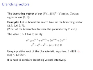
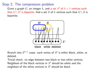
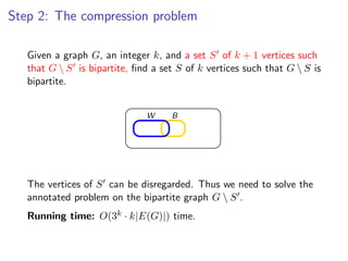
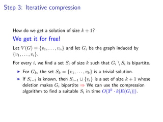
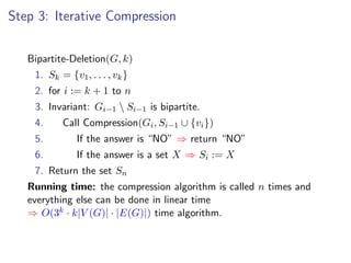
![Proof
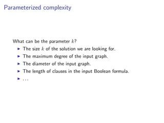
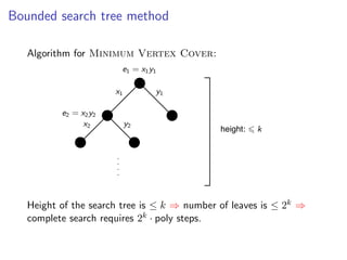
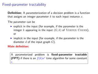
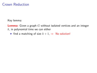
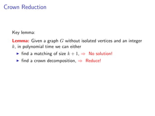
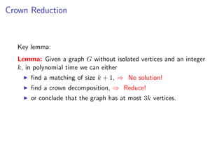
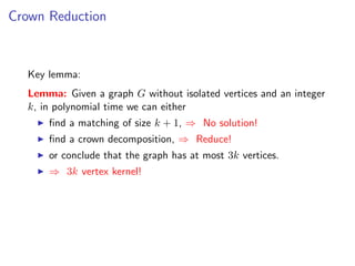
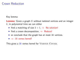
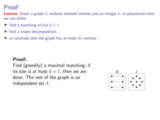
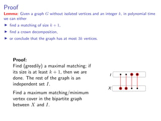
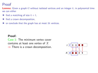
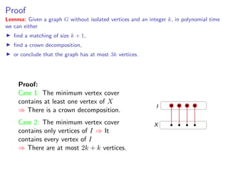
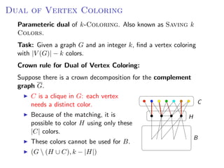
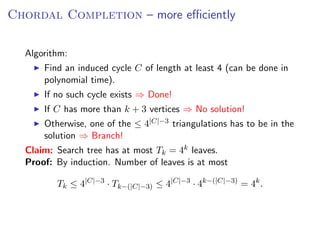
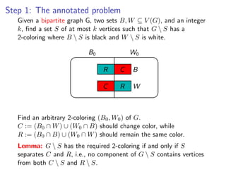
Lemma: Given a graph G without isolated vertices and an integer k, in polynomial time
we can either
find a matching of size k + 1,
find a crown decomposition,
or conclude that the graph has at most 3k vertices.
For the proof, we need the classical K˝nig’s Theorem.
o
τ (G) : size of the minimum vertex cover
ν(G) : size of the maximum matching (independent set of
edges)
Theorem: [K˝nig, 1931] If G is bipartite, then
o
τ (G) = ν(G)](https://image.slidesharecdn.com/20110319parameterizedalgorithmsfominlecture01-02-110324035957-phpapp01/85/20110319-parameterized-algorithms_fomin_lecture01-02-48-320.jpg)
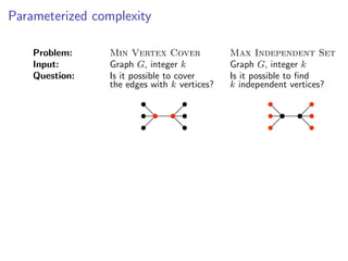
![Sunflower lemma
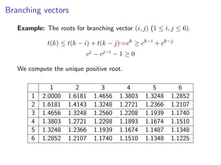
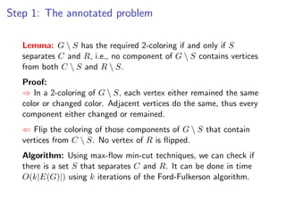
Sunflower lemma
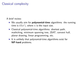
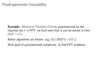
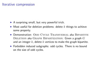
Definition: Sets S1 , S2 , . . . , Sk form a sunflower if the sets
Si Definition:S2 ∩S·1 ,· S2∩... , k ) form a sunflower if the sets
(S1 ∩ Sets · , S Sk are disjoint.
Si (S1 ∩ S2 ∩ · · · ∩ Sk ) are disjoint.
petals
center
˝
Lemma: [Erdos and Rado, 1960] If the size of a set system is greater than
(p − 1)d · d! and it contains only sets of size at most d , then the system contains a
Lemma: [Erd˝petals. Furthermore, in thisIf the size sunflower can be foundis
sunflower with p
os and Rado, 1960] case such a of a set system in
greater than (p − 1)d · d! and it contains only sets of size at most d,
polynomial time.
then the system contains a sunflower with p petals. Furthermore,
in this case such a sunflower can be found in polynomial time. Fixed Parameter Algorithms – p.27/98](https://image.slidesharecdn.com/20110319parameterizedalgorithmsfominlecture01-02-110324035957-phpapp01/85/20110319-parameterized-algorithms_fomin_lecture01-02-58-320.jpg)
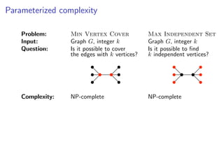
![Sunflowers and d-Hitting Set
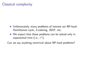
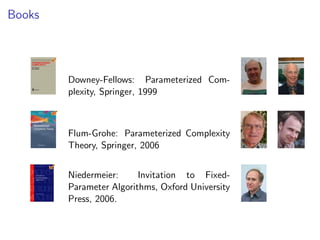
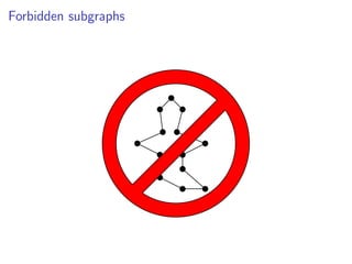
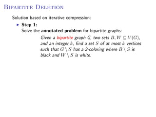
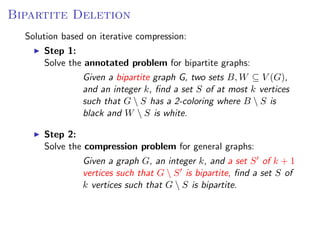
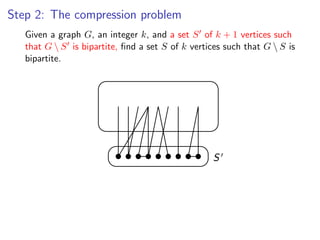
d-Hitting Set: Given a collection S of sets of size at most d Sunflower lemma
and an integer k, find a set S of k elements that intersects every
set of S. Definition: Sets S , S , ... , S form a sunflower if the sets
1 2 k
Si (S1 ∩ S2 ∩ · · · ∩ Sk ) are disjoint.
petals
center
˝
Lemma: [Erdos and Rado, 1960] If the size of a set system is greater than
(p − 1)d · d! and it contains only sets of size at most d , then the system contains a
Reduction Rule: p petals. Furthermore, inform a sunflower, be found in
sunflower with If k + 1 sets this case such a sunflower can then remove
these sets polynomialS and add the center C to S (S does not hit one
from time.
of the petals, thus it has to hit the center). Fixed Parameter Algorithms – p.27/98
Note: if the center is empty (the sets are disjoint), then there is no
solution.
If the rule cannot be applied, then there are at most O(k d ) sets.](https://image.slidesharecdn.com/20110319parameterizedalgorithmsfominlecture01-02-110324035957-phpapp01/85/20110319-parameterized-algorithms_fomin_lecture01-02-59-320.jpg)
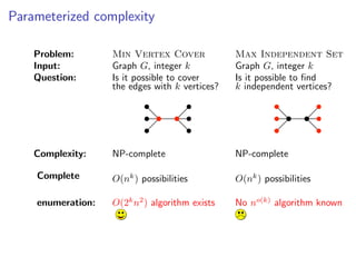
![Sunflowers and d-Hitting Set
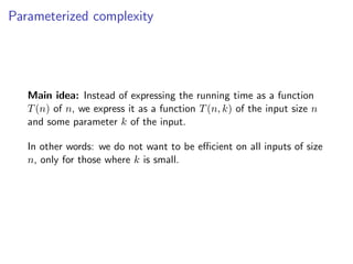
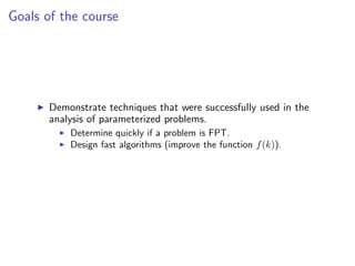
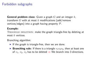
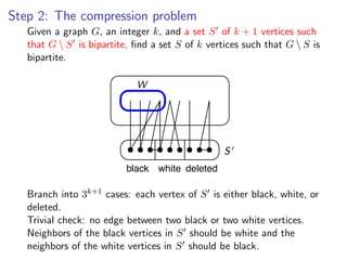
d-Hitting Set: Given a collection S of sets of size at most d Sunflower lemma
and an integer k, find a set S of k elements that intersects every
set of S. Definition: Sets S , S , ... , S form a sunflower if the sets
1 2 k
Si (S1 ∩ S2 ∩ · · · ∩ Sk ) are disjoint.
petals
center
˝
Lemma: [Erdos and Rado, 1960] If the size of a set system is greater than
(p − 1)d · d! and it contains only sets of size at most d , then the system contains a
Reduction Rule (variant): Suppose such a sunflower cank + 1insets form a
sunflower with p petals. Furthermore, in this case more than be found
sunflower. polynomial time.
If the sets are disjoint ⇒ No solution. Fixed Parameter Algorithms – p.27/98
Otherwise, keep only k + 1 of the sets.
If the rule cannot be applied, then there are at most O(k d ) sets.](https://image.slidesharecdn.com/20110319parameterizedalgorithmsfominlecture01-02-110324035957-phpapp01/85/20110319-parameterized-algorithms_fomin_lecture01-02-60-320.jpg)


![k-Path
Assign colors from [k] to vertices V (G) {s, t} uniformly and
Assign colors from [k] to vertices V (G ) {s, t} uniformly and independently at
independently at random.
random.
s t](https://image.slidesharecdn.com/20110319parameterizedalgorithmsfominlecture01-02-110324035957-phpapp01/85/20110319-parameterized-algorithms_fomin_lecture01-02-109-320.jpg)
![k-Path
Assign colors from [k] to vertices V t} {s, t} uniformly and
Assign colors from [k] to vertices V (G ) {s,(G)uniformly and independently
random. independently at random.
s t](https://image.slidesharecdn.com/20110319parameterizedalgorithmsfominlecture01-02-110324035957-phpapp01/85/20110319-parameterized-algorithms_fomin_lecture01-02-110-320.jpg)
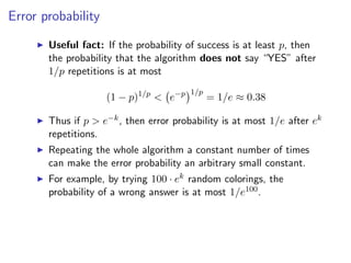
![k-Path
Assign colors from [k]from [k] to V (G ) {s, (G) {s, t} and independently at
Assign colors to vertices vertices V t} uniformly uniformly and
independently at random.
random.
s t
there if there is a s -t path: a path: a path where appears exactly
Check ifCheck is a colorful colorful s-tpath where each coloreach color
once onappears exactly once output “YES” or vertices; output “YES”
the internal vertices; on the internal “NO”.
or “NO”.
Fixed Parameter Algorithms – p.69](https://image.slidesharecdn.com/20110319parameterizedalgorithmsfominlecture01-02-110324035957-phpapp01/85/20110319-parameterized-algorithms_fomin_lecture01-02-111-320.jpg)
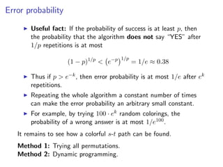
![k-Path
Assign colors from [k]from [k] to V (G ) {s, (G) {s, t} and independently at
Assign colors to vertices vertices V t} uniformly uniformly and
independently at random.
random.
s t
there if there is a s -t path: a path: a path where appears exactly
Check ifCheck is a colorful colorful s-tpath where each coloreach color
once onappears exactly once output “YES” or vertices; output “YES”
the internal vertices; on the internal “NO”.
or “NO”.
If there is no s-t k-path: no such colorful path exists ⇒ “NO”.
If there is an s-t k-path: the probability that such a path is
colorful is
k! ( k )k
> e k = e−k ,
kk k
thus the algorithm outputs “YES” with at least that
probability.
Fixed Parameter Algorithms – p.69](https://image.slidesharecdn.com/20110319parameterizedalgorithmsfominlecture01-02-110324035957-phpapp01/85/20110319-parameterized-algorithms_fomin_lecture01-02-112-320.jpg)
![Method 2: Dynamic Programming
We introduce 2k · |V (G)| Boolean variables:
x(v, C) = TRUE for some v ∈ V (G) and C ⊆ [k]
There is an s-v path where each color in C appears
exactly once and no other color appears.](https://image.slidesharecdn.com/20110319parameterizedalgorithmsfominlecture01-02-110324035957-phpapp01/85/20110319-parameterized-algorithms_fomin_lecture01-02-119-320.jpg)
![Method 2: Dynamic Programming
We introduce 2k · |V (G)| Boolean variables:
x(v, C) = TRUE for some v ∈ V (G) and C ⊆ [k]
There is an s-v path where each color in C appears
exactly once and no other color appears.
Clearly, x(s, ∅) = TRUE. Recurrence for vertex v with color r:
x(v, C) = x(u, C {r})
uv∈E(G)](https://image.slidesharecdn.com/20110319parameterizedalgorithmsfominlecture01-02-110324035957-phpapp01/85/20110319-parameterized-algorithms_fomin_lecture01-02-120-320.jpg)
![Method 2: Dynamic Programming
We introduce 2k · |V (G)| Boolean variables:
x(v, C) = TRUE for some v ∈ V (G) and C ⊆ [k]
There is an s-v path where each color in C appears
exactly once and no other color appears.
Clearly, x(s, ∅) = TRUE. Recurrence for vertex v with color r:
x(v, C) = x(u, C {r})
uv∈E(G)
If we know every x(v, C) with |C| = i, then we can determine
every x(v, C) with |C| = i + 1 ⇒ All the values can be determined
in time O(2k · |E(G)|).
There is a colorful s-t path ⇐⇒ x(v, [k]) = TRUE for some
neighbor of t.](https://image.slidesharecdn.com/20110319parameterizedalgorithmsfominlecture01-02-110324035957-phpapp01/85/20110319-parameterized-algorithms_fomin_lecture01-02-121-320.jpg)
![Derandomization
Using Method 2, we obtain a O∗ ((2e)k ) time algorithm with
constant error probability. How to make it deterministic?
Definition: A family H of functions [n] → [k] is a k-perfect
family of hash functions if for every S ⊆ [n] with |S| = k, there is
a h ∈ H such that h(x) = h(y) for any x, y ∈ S, x = y.](https://image.slidesharecdn.com/20110319parameterizedalgorithmsfominlecture01-02-110324035957-phpapp01/85/20110319-parameterized-algorithms_fomin_lecture01-02-122-320.jpg)
![Derandomization
Using Method 2, we obtain a O∗ ((2e)k ) time algorithm with
constant error probability. How to make it deterministic?
Definition: A family H of functions [n] → [k] is a k-perfect
family of hash functions if for every S ⊆ [n] with |S| = k, there is
a h ∈ H such that h(x) = h(y) for any x, y ∈ S, x = y.
Instead of trying O(ek ) random colorings, we go through a
k-perfect family H of functions V (G) → [k]. If there is a solution
⇒ The internal vertices S are colorful for at least one h ∈ H ⇒
Algorithm outputs “YES”.](https://image.slidesharecdn.com/20110319parameterizedalgorithmsfominlecture01-02-110324035957-phpapp01/85/20110319-parameterized-algorithms_fomin_lecture01-02-123-320.jpg)
![Derandomization
Using Method 2, we obtain a O∗ ((2e)k ) time algorithm with
constant error probability. How to make it deterministic?
Definition: A family H of functions [n] → [k] is a k-perfect
family of hash functions if for every S ⊆ [n] with |S| = k, there is
a h ∈ H such that h(x) = h(y) for any x, y ∈ S, x = y.
Instead of trying O(ek ) random colorings, we go through a
k-perfect family H of functions V (G) → [k]. If there is a solution
⇒ The internal vertices S are colorful for at least one h ∈ H ⇒
Algorithm outputs “YES”.
Theorem: There is a k-perfect family of functions [n] → [k]
having size 2O(k) log n
(and can be constructed in time polynomial in the size of the
family).
⇒ There is a deterministic 2O(k) · nO(1) time algorithm for the
k-Path problem.](https://image.slidesharecdn.com/20110319parameterizedalgorithmsfominlecture01-02-110324035957-phpapp01/85/20110319-parameterized-algorithms_fomin_lecture01-02-124-320.jpg)
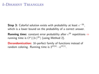
![k-Disjoint Triangles
Task: Given a graph G and an integer k, find k vertex disjoint
triangles.
Step 1: Choose a random coloring V (G) → [3k].](https://image.slidesharecdn.com/20110319parameterizedalgorithmsfominlecture01-02-110324035957-phpapp01/85/20110319-parameterized-algorithms_fomin_lecture01-02-125-320.jpg)
![k-Disjoint Triangles
Task: Given a graph G and an integer k, find k vertex disjoint
triangles.
Step 1: Choose a random coloring V (G) → [3k].
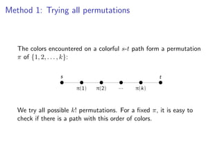
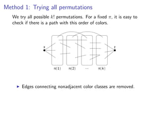
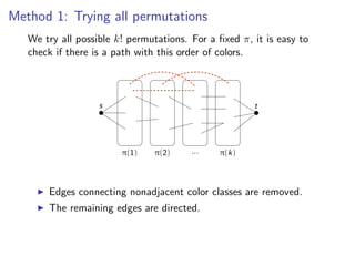
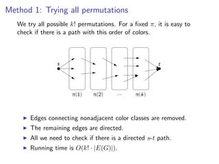
Step 2: Check if there is a colorful solution, where the 3k vertices
of the k triangles use distinct colors.
Method 1: Try every permutation π of [3k] and check if
there are triangles with colors (π(1), π(2), π(3)),
(π(4), π(5), π(6)), . . .
Method 2: Dynamic programming. For C ⊆ [3k] and
|C| = 3i, let x(C) = TRUE if and only if there are |C|/3
disjoint triangles using exactly the colors in C.
x(C) = (x(C {c1 , c2 , c3 }) ∧ ∃ with colors c1 , c2 , c3 )
{c1 ,c2 ,c3 }⊆C](https://image.slidesharecdn.com/20110319parameterizedalgorithmsfominlecture01-02-110324035957-phpapp01/85/20110319-parameterized-algorithms_fomin_lecture01-02-126-320.jpg)

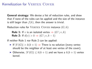
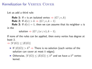
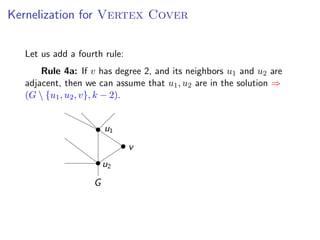
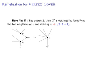
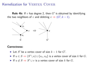
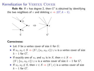
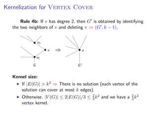
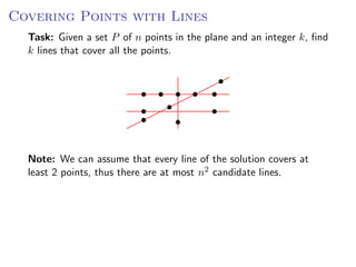
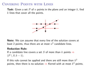
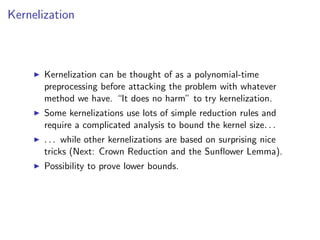
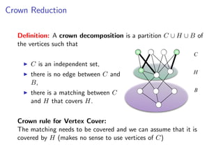
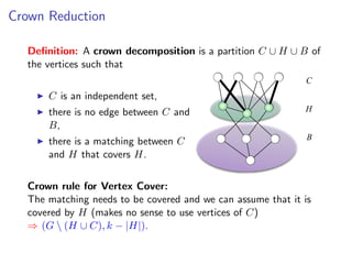
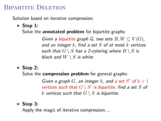
The document discusses kernelization, which is a polynomial-time transformation that maps an instance of a parameterized problem to an equivalent instance whose size is bounded by a function of the parameter k. If a problem admits a kernelization algorithm, then it is fixed-parameter tractable. The document introduces kernelization and provides definitions. It also notes that every fixed-parameter tractable problem has a kernelization algorithm.