graphs of first degree functions

1. First Degree Functions

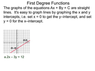
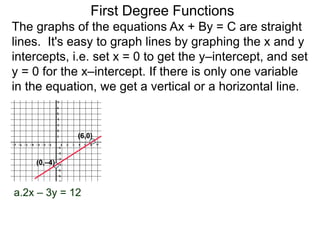
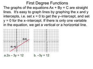
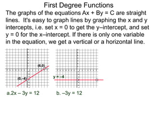
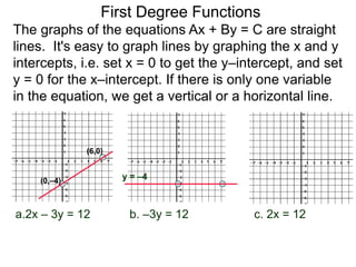
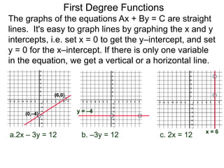
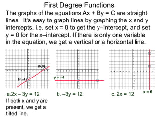
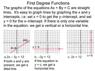
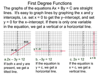
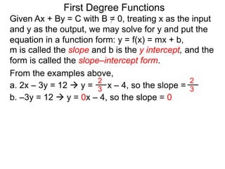
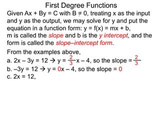
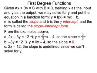
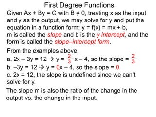
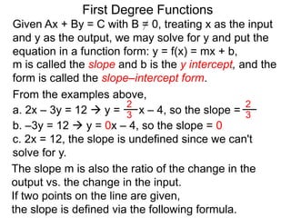
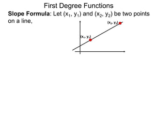
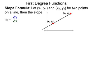
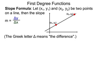
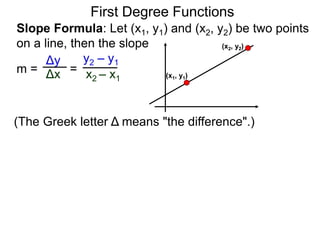
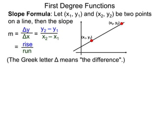
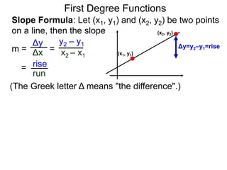
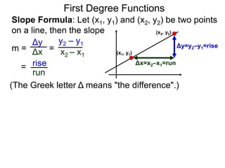
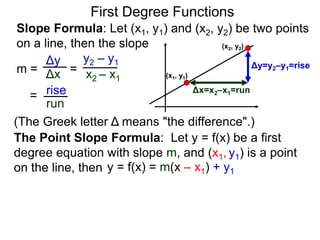
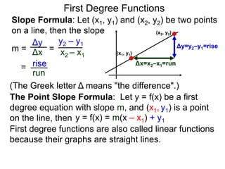
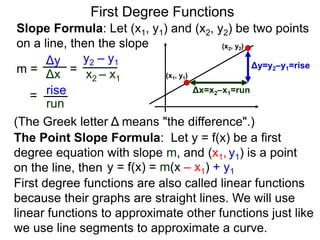
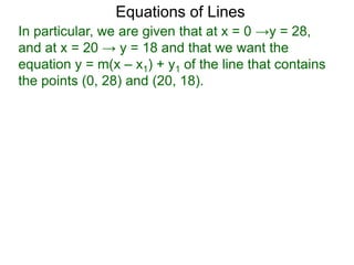
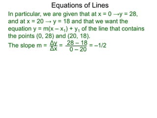
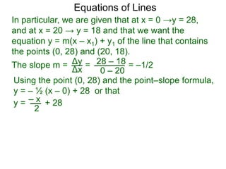
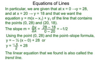
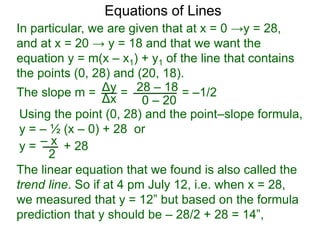
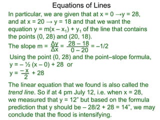
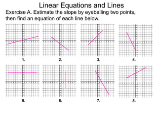
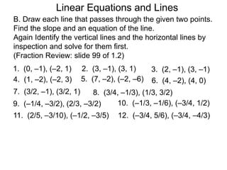
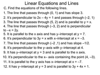
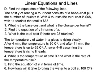
2. First Degree Functions
Most mathematical functions used in the real world are
“composed” with members from the following three
groups of formulas.

3. Most mathematical functions used in the real world are
“composed” with members from the following three
groups of formulas.
* The algebraic family – these are polynomials,
rational expressions and roots, etc..
First Degree Functions

4. Most mathematical functions used in the real world are
“composed” with members from the following three
groups of formulas.
* The algebraic family – these are polynomials,
rational expressions and roots, etc..
* The trigonometric family – these are sin(x),
cos(x), .. etc that come from line measurements.
First Degree Functions

5. Most mathematical functions used in the real world are
“composed” with members from the following three
groups of formulas.
* The algebraic family – these are polynomials,
rational expressions and roots, etc..
* The trigonometric family – these are sin(x),
cos(x), .. etc that come from line measurements.
* The exponential–log family – these are ex and ln(x)
that come from exponential contexts.
First Degree Functions

6. Most mathematical functions used in the real world are
“composed” with members from the following three
groups of formulas.
* The algebraic family – these are polynomials,
rational expressions and roots, etc..
* The trigonometric family – these are sin(x),
cos(x), .. etc that come from line measurements.
* The exponential–log family – these are ex and ln(x)
that come from exponential contexts.
Degree 1 or linear functions: f(x) = mx + b and
degree 2 or quadratic functions: f(x) = ax2 + bx + c
are especially important.
First Degree Functions

7. Most mathematical functions used in the real world are
“composed” with members from the following three
groups of formulas.
* The algebraic family – these are polynomials,
rational expressions and roots, etc..
* The trigonometric family – these are sin(x),
cos(x), .. etc that come from line measurements.
* The exponential–log family – these are ex and ln(x)
that come from exponential contexts.
Degree 1 or linear functions: f(x) = mx + b and
degree 2 or quadratic functions: f(x) = ax2 + bx + c
are especially important.
First Degree Functions
We review below the basics of linear equations and
linear functions.

8. First Degree Functions
The algebraic family
The exponential–log familyThe trigonometric family
Below is the MS Win-10 desktop scientific calculator,
a typical scientific calculator input panel:

9. The graphs of the equations Ax + By = C are straight
lines.
First Degree Functions

10. The graphs of the equations Ax + By = C are straight
lines. It's easy to graph lines by graphing the x and y
intercepts,
First Degree Functions

11. a.2x – 3y = 12
The graphs of the equations Ax + By = C are straight
lines. It's easy to graph lines by graphing the x and y
intercepts,
First Degree Functions

12. a.2x – 3y = 12
The graphs of the equations Ax + By = C are straight
lines. It's easy to graph lines by graphing the x and y
intercepts, i.e. set x = 0 to get the y–intercept,
(0,–4)
First Degree Functions

13. a.2x – 3y = 12
The graphs of the equations Ax + By = C are straight
lines. It's easy to graph lines by graphing the x and y
intercepts, i.e. set x = 0 to get the y–intercept, and set
y = 0 for the x–intercept.
(6,0)
(0,–4)
First Degree Functions

14. a.2x – 3y = 12
The graphs of the equations Ax + By = C are straight
lines. It's easy to graph lines by graphing the x and y
intercepts, i.e. set x = 0 to get the y–intercept, and set
y = 0 for the x–intercept.
(6,0)
(0,–4)
First Degree Functions

15. a.2x – 3y = 12
The graphs of the equations Ax + By = C are straight
lines. It's easy to graph lines by graphing the x and y
intercepts, i.e. set x = 0 to get the y–intercept, and set
y = 0 for the x–intercept. If there is only one variable
in the equation, we get a vertical or a horizontal line.
(6,0)
(0,–4)
First Degree Functions

16. a.2x – 3y = 12 b. –3y = 12
The graphs of the equations Ax + By = C are straight
lines. It's easy to graph lines by graphing the x and y
intercepts, i.e. set x = 0 to get the y–intercept, and set
y = 0 for the x–intercept. If there is only one variable
in the equation, we get a vertical or a horizontal line.
(6,0)
(0,–4)
First Degree Functions

17. a.2x – 3y = 12 b. –3y = 12
The graphs of the equations Ax + By = C are straight
lines. It's easy to graph lines by graphing the x and y
intercepts, i.e. set x = 0 to get the y–intercept, and set
y = 0 for the x–intercept. If there is only one variable
in the equation, we get a vertical or a horizontal line.
(6,0)
(0,–4) y = –4
First Degree Functions

18. a.2x – 3y = 12 b. –3y = 12 c. 2x = 12
The graphs of the equations Ax + By = C are straight
lines. It's easy to graph lines by graphing the x and y
intercepts, i.e. set x = 0 to get the y–intercept, and set
y = 0 for the x–intercept. If there is only one variable
in the equation, we get a vertical or a horizontal line.
(6,0)
(0,–4) y = –4
First Degree Functions

19. a.2x – 3y = 12 b. –3y = 12 c. 2x = 12
The graphs of the equations Ax + By = C are straight
lines. It's easy to graph lines by graphing the x and y
intercepts, i.e. set x = 0 to get the y–intercept, and set
y = 0 for the x–intercept. If there is only one variable
in the equation, we get a vertical or a horizontal line.
(6,0)
(0,–4) y = –4
x = 6
First Degree Functions

20. a.2x – 3y = 12 b. –3y = 12 c. 2x = 12
If both x and y are
present, we get a
tilted line.
The graphs of the equations Ax + By = C are straight
lines. It's easy to graph lines by graphing the x and y
intercepts, i.e. set x = 0 to get the y–intercept, and set
y = 0 for the x–intercept. If there is only one variable
in the equation, we get a vertical or a horizontal line.
(6,0)
(0,–4) y = –4
x = 6
First Degree Functions

21. a.2x – 3y = 12 b. –3y = 12 c. 2x = 12
If both x and y are
present, we get a
tilted line.
If the equation is
y = c, we get a
horizontal line.
The graphs of the equations Ax + By = C are straight
lines. It's easy to graph lines by graphing the x and y
intercepts, i.e. set x = 0 to get the y–intercept, and set
y = 0 for the x–intercept. If there is only one variable
in the equation, we get a vertical or a horizontal line.
(6,0)
(0,–4) y = –4
x = 6
First Degree Functions

22. a.2x – 3y = 12 b. –3y = 12 c. 2x = 12
If both x and y are
present, we get a
tilted line.
If the equation is
y = c, we get a
horizontal line.
The graphs of the equations Ax + By = C are straight
lines. It's easy to graph lines by graphing the x and y
intercepts, i.e. set x = 0 to get the y–intercept, and set
y = 0 for the x–intercept. If there is only one variable
in the equation, we get a vertical or a horizontal line.
(6,0)
(0,–4) y = –4
x = 6
If the equation is
x = c, we get a
vertical line.
First Degree Functions

23. First Degree Functions
Given Ax + By = C with B = 0,

24. First Degree Functions
Given Ax + By = C with B = 0, treating x as the input
and y as the output, we may solve for y and put the
equation in a function form: y = f(x) = mx + b,

25. First Degree Functions
Given Ax + By = C with B = 0, treating x as the input
and y as the output, we may solve for y and put the
equation in a function form: y = f(x) = mx + b,
m is called the slope and b is the y intercept,

26. First Degree Functions
Given Ax + By = C with B = 0, treating x as the input
and y as the output, we may solve for y and put the
equation in a function form: y = f(x) = mx + b,
m is called the slope and b is the y intercept, and the
form is called the slope–intercept form.

27. First Degree Functions
Given Ax + By = C with B = 0, treating x as the input
and y as the output, we may solve for y and put the
equation in a function form: y = f(x) = mx + b,
m is called the slope and b is the y intercept, and the
form is called the slope–intercept form.
From the examples above,
a. 2x – 3y = 12 

28. First Degree Functions
Given Ax + By = C with B = 0, treating x as the input
and y as the output, we may solve for y and put the
equation in a function form: y = f(x) = mx + b,
m is called the slope and b is the y intercept, and the
form is called the slope–intercept form.
2
3
2
3
From the examples above,
a. 2x – 3y = 12  y = x – 4, so the slope =

29. First Degree Functions
Given Ax + By = C with B = 0, treating x as the input
and y as the output, we may solve for y and put the
equation in a function form: y = f(x) = mx + b,
m is called the slope and b is the y intercept, and the
form is called the slope–intercept form.
2
3
2
3
From the examples above,
a. 2x – 3y = 12  y = x – 4, so the slope =
b. –3y = 12

30. First Degree Functions
Given Ax + By = C with B = 0, treating x as the input
and y as the output, we may solve for y and put the
equation in a function form: y = f(x) = mx + b,
m is called the slope and b is the y intercept, and the
form is called the slope–intercept form.
2
3
2
3
From the examples above,
a. 2x – 3y = 12  y = x – 4, so the slope =
b. –3y = 12  y = 0x – 4, so the slope = 0

31. First Degree Functions
Given Ax + By = C with B = 0, treating x as the input
and y as the output, we may solve for y and put the
equation in a function form: y = f(x) = mx + b,
m is called the slope and b is the y intercept, and the
form is called the slope–intercept form.
2
3
2
3
From the examples above,
a. 2x – 3y = 12  y = x – 4, so the slope =
b. –3y = 12  y = 0x – 4, so the slope = 0
c. 2x = 12,

32. First Degree Functions
Given Ax + By = C with B = 0, treating x as the input
and y as the output, we may solve for y and put the
equation in a function form: y = f(x) = mx + b,
m is called the slope and b is the y intercept, and the
form is called the slope–intercept form.
2
3
2
3
From the examples above,
a. 2x – 3y = 12  y = x – 4, so the slope =
b. –3y = 12  y = 0x – 4, so the slope = 0
c. 2x = 12, the slope is undefined since we can't
solve for y.

33. First Degree Functions
Given Ax + By = C with B = 0, treating x as the input
and y as the output, we may solve for y and put the
equation in a function form: y = f(x) = mx + b,
m is called the slope and b is the y intercept, and the
form is called the slope–intercept form.
The slope m is also the ratio of the change in the
output vs. the change in the input.
2
3
2
3
From the examples above,
a. 2x – 3y = 12  y = x – 4, so the slope =
b. –3y = 12  y = 0x – 4, so the slope = 0
c. 2x = 12, the slope is undefined since we can't
solve for y.

34. First Degree Functions
Given Ax + By = C with B = 0, treating x as the input
and y as the output, we may solve for y and put the
equation in a function form: y = f(x) = mx + b,
m is called the slope and b is the y intercept, and the
form is called the slope–intercept form.
The slope m is also the ratio of the change in the
output vs. the change in the input.
If two points on the line are given,
the slope is defined via the following formula.
2
3
2
3
From the examples above,
a. 2x – 3y = 12  y = x – 4, so the slope =
b. –3y = 12  y = 0x – 4, so the slope = 0
c. 2x = 12, the slope is undefined since we can't
solve for y.

35. Slope Formula: Let (x1, y1) and (x2, y2) be two points
on a line,
First Degree Functions
(x1, y1)
(x2, y2)

36. Slope Formula: Let (x1, y1) and (x2, y2) be two points
on a line, then the slope
Δy
Δxm =
First Degree Functions
(x1, y1)
(x2, y2)

37. Slope Formula: Let (x1, y1) and (x2, y2) be two points
on a line, then the slope
Δy
Δxm =
First Degree Functions
(The Greek letter Δ means "the difference".)
(x1, y1)
(x2, y2)

38. Slope Formula: Let (x1, y1) and (x2, y2) be two points
on a line, then the slope
Δy
Δx
y2 – y1
x2 – x1
m = =
First Degree Functions
(The Greek letter Δ means "the difference".)
(x1, y1)
(x2, y2)

39. Slope Formula: Let (x1, y1) and (x2, y2) be two points
on a line, then the slope
Δy
Δx
y2 – y1
x2 – x1
m =
rise
run
=
=
First Degree Functions
(The Greek letter Δ means "the difference".)
(x1, y1)
(x2, y2)

40. Slope Formula: Let (x1, y1) and (x2, y2) be two points
on a line, then the slope
Δy
Δx
y2 – y1
x2 – x1
m =
rise
run
=
= (x1, y1)
(x2, y2)
First Degree Functions
(The Greek letter Δ means "the difference".)

41. Slope Formula: Let (x1, y1) and (x2, y2) be two points
on a line, then the slope
Δy
Δx
y2 – y1
x2 – x1
m =
rise
run
=
= (x1, y1)
(x2, y2)
Δy=y2–y1=rise
First Degree Functions
(The Greek letter Δ means "the difference".)

42. Slope Formula: Let (x1, y1) and (x2, y2) be two points
on a line, then the slope
Δy
Δx
y2 – y1
x2 – x1
m =
rise
run
=
= (x1, y1)
(x2, y2)
Δy=y2–y1=rise
Δx=x2–x1=run
First Degree Functions
(The Greek letter Δ means "the difference".)

43. Slope Formula: Let (x1, y1) and (x2, y2) be two points
on a line, then the slope
Δy
Δx
y2 – y1
x2 – x1
m =
rise
run
=
= (x1, y1)
(x2, y2)
Δy=y2–y1=rise
Δx=x2–x1=run
The Point Slope Formula: Let y = f(x) be a first
degree equation with slope m, and (x1, y1) is a point
on the line, then y = f(x) = m(x – x1) + y1
First Degree Functions
(The Greek letter Δ means "the difference".)

44. Slope Formula: Let (x1, y1) and (x2, y2) be two points
on a line, then the slope
Δy
Δx
y2 – y1
x2 – x1
m =
rise
run
=
= (x1, y1)
(x2, y2)
Δy=y2–y1=rise
Δx=x2–x1=run
The Point Slope Formula: Let y = f(x) be a first
degree equation with slope m, and (x1, y1) is a point
on the line, then y = f(x) = m(x – x1) + y1
First degree functions are also called linear functions
because their graphs are straight lines.
First Degree Functions
(The Greek letter Δ means "the difference".)

45. Slope Formula: Let (x1, y1) and (x2, y2) be two points
on a line, then the slope
Δy
Δx
y2 – y1
x2 – x1
m =
rise
run
=
= (x1, y1)
(x2, y2)
Δy=y2–y1=rise
Δx=x2–x1=run
The Point Slope Formula: Let y = f(x) be a first
degree equation with slope m, and (x1, y1) is a point
on the line, then y = f(x) = m(x – x1) + y1
First degree functions are also called linear functions
because their graphs are straight lines. We will use
linear functions to approximate other functions just like
we use line segments to approximate a curve.
First Degree Functions
(The Greek letter Δ means "the difference".)

46. Linear Equations and Lines
Example A. A river floods regularly, and on a rock by
the river there is a mark indicating the highest point
the water level ever recorded.
At 12 pm July 11, the water level is 28 inches below
this mark. At 8 am July 12 the water is 18 inches
below this mark.

47. Linear Equations and Lines
Example A. A river floods regularly, and on a rock by
the river there is a mark indicating the highest point
the water level ever recorded.
At 12 pm July 11, the water level is 28 inches below
this mark. At 8 am July 12 the water is 18 inches
below this mark. Let x = time,
y = distance between the water level and the mark.
Find the linear function y = f(x) = mx + b
of the distance y in terms of time x.

48. Linear Equations and Lines
Example A. A river floods regularly, and on a rock by
the river there is a mark indicating the highest point
the water level ever recorded.
At 12 pm July 11, the water level is 28 inches below
this mark. At 8 am July 12 the water is 18 inches
below this mark. Let x = time,
y = distance between the water level and the mark.
Find the linear function y = f(x) = mx + b
of the distance y in terms of time x.
Since how the time was measured is not specified,
we may select the stating time 0 to be time of the
first observation.

49. Linear Equations and Lines
Example A. A river floods regularly, and on a rock by
the river there is a mark indicating the highest point
the water level ever recorded.
At 12 pm July 11, the water level is 28 inches below
this mark. At 8 am July 12 the water is 18 inches
below this mark. Let x = time,
y = distance between the water level and the mark.
Find the linear function y = f(x) = mx + b
of the distance y in terms of time x.
Since how the time was measured is not specified,
we may select the stating time 0 to be time of the
first observation.
By setting x = 0 (hr) at 12 pm July 11,
then x = 20 at 8 am of July 12.

50. Equations of Lines
In particular, we are given that at x = 0 →y = 28,
and at x = 20 → y = 18

51. Equations of Lines
In particular, we are given that at x = 0 →y = 28,
and at x = 20 → y = 18 and that we want the
equation y = m(x – x1) + y1 of the line that contains
the points (0, 28) and (20, 18).

52. Δy
Δx
28 – 18
0 – 20
Equations of Lines
In particular, we are given that at x = 0 →y = 28,
and at x = 20 → y = 18 and that we want the
equation y = m(x – x1) + y1 of the line that contains
the points (0, 28) and (20, 18).
=The slope m = = –1/2

53. Using the point (0, 28) and the point–slope formula,
y = – ½ (x – 0) + 28 or that
Δy
Δx
28 – 18
0 – 20
Equations of Lines
In particular, we are given that at x = 0 →y = 28,
and at x = 20 → y = 18 and that we want the
equation y = m(x – x1) + y1 of the line that contains
the points (0, 28) and (20, 18).
=The slope m = = –1/2
– xy = + 28
2

54. Using the point (0, 28) and the point–slope formula,
y = – ½ (x – 0) + 28 or
Δy
Δx
28 – 18
0 – 20
Equations of Lines
In particular, we are given that at x = 0 →y = 28,
and at x = 20 → y = 18 and that we want the
equation y = m(x – x1) + y1 of the line that contains
the points (0, 28) and (20, 18).
=The slope m = = –1/2
– xy = + 28
2
The linear equation that we found is also called the
trend line.

55. Using the point (0, 28) and the point–slope formula,
y = – ½ (x – 0) + 28 or
Δy
Δx
28 – 18
0 – 20
Equations of Lines
In particular, we are given that at x = 0 →y = 28,
and at x = 20 → y = 18 and that we want the
equation y = m(x – x1) + y1 of the line that contains
the points (0, 28) and (20, 18).
=The slope m = = –1/2
– xy = + 28
2
The linear equation that we found is also called the
trend line. So if at 4 pm July 12, i.e. when x = 28,
we measured that y = 12”

56. Using the point (0, 28) and the point–slope formula,
y = – ½ (x – 0) + 28 or
Δy
Δx
28 – 18
0 – 20
Equations of Lines
In particular, we are given that at x = 0 →y = 28,
and at x = 20 → y = 18 and that we want the
equation y = m(x – x1) + y1 of the line that contains
the points (0, 28) and (20, 18).
=The slope m = = –1/2
– xy = + 28
2
The linear equation that we found is also called the
trend line. So if at 4 pm July 12, i.e. when x = 28,
we measured that y = 12” but based on the formula
prediction that y should be – 28/2 + 28 = 14”,

57. Using the point (0, 28) and the point–slope formula,
y = – ½ (x – 0) + 28 or
Δy
Δx
28 – 18
0 – 20
Equations of Lines
In particular, we are given that at x = 0 →y = 28,
and at x = 20 → y = 18 and that we want the
equation y = m(x – x1) + y1 of the line that contains
the points (0, 28) and (20, 18).
=The slope m = = –1/2
– xy = + 28
2
The linear equation that we found is also called the
trend line. So if at 4 pm July 12, i.e. when x = 28,
we measured that y = 12” but based on the formula
prediction that y should be – 28/2 + 28 = 14”, we may
conclude that the flood is intensifying.

58. More Facts on Slopes:
First Degree Functions

59. More Facts on Slopes:
• Parallel lines have the same slope.
First Degree Functions

60. More Facts on Slopes:
• Parallel lines have the same slope.
• Slopes of perpendicular lines are the negative
reciprocal of each other.
First Degree Functions

61. More Facts on Slopes:
• Parallel lines have the same slope.
• Slopes of perpendicular lines are the negative
reciprocal of each other.
Example B. Find the equation of the line L that
passes through (2, –4) and is perpendicular to
4x – 3y = 5.
First Degree Functions

62. More Facts on Slopes:
• Parallel lines have the same slope.
• Slopes of perpendicular lines are the negative
reciprocal of each other.
Example B. Find the equation of the line L that
passes through (2, –4) and is perpendicular to
4x – 3y = 5.
Solve for y to find the slope of 4x – 3y = 5
First Degree Functions

63. More Facts on Slopes:
• Parallel lines have the same slope.
• Slopes of perpendicular lines are the negative
reciprocal of each other.
Example B. Find the equation of the line L that
passes through (2, –4) and is perpendicular to
4x – 3y = 5.
Solve for y to find the slope of 4x – 3y = 5
4x – 5 = 3y
First Degree Functions

64. More Facts on Slopes:
• Parallel lines have the same slope.
• Slopes of perpendicular lines are the negative
reciprocal of each other.
Example B. Find the equation of the line L that
passes through (2, –4) and is perpendicular to
4x – 3y = 5.
Solve for y to find the slope of 4x – 3y = 5
4x – 5 = 3y
4x/3 – 5/3 = y
First Degree Functions

65. More Facts on Slopes:
• Parallel lines have the same slope.
• Slopes of perpendicular lines are the negative
reciprocal of each other.
Example B. Find the equation of the line L that
passes through (2, –4) and is perpendicular to
4x – 3y = 5.
Solve for y to find the slope of 4x – 3y = 5
4x – 5 = 3y
4x/3 – 5/3 = y
Hence the slope of 4x – 2y = 5 is 4/3.
First Degree Functions

66. More Facts on Slopes:
• Parallel lines have the same slope.
• Slopes of perpendicular lines are the negative
reciprocal of each other.
Example B. Find the equation of the line L that
passes through (2, –4) and is perpendicular to
4x – 3y = 5.
Solve for y to find the slope of 4x – 3y = 5
4x – 5 = 3y
4x/3 – 5/3 = y
Hence the slope of 4x – 2y = 5 is 4/3.
Therefore L has slope –3/4.
First Degree Functions

67. More Facts on Slopes:
• Parallel lines have the same slope.
• Slopes of perpendicular lines are the negative
reciprocal of each other.
Example B. Find the equation of the line L that
passes through (2, –4) and is perpendicular to
4x – 3y = 5.
Solve for y to find the slope of 4x – 3y = 5
4x – 5 = 3y
4x/3 – 5/3 = y
Hence the slope of 4x – 2y = 5 is 4/3.
Therefore L has slope –3/4. So the equation of L is
First Degree Functions
y = (–3/4)(x – 2) + (–4) or y = –3x/4 – 5/2.

68. Linear Equations and Lines
Exercise A. Estimate the slope by eyeballing two points,
then find an equation of each line below.
1. 2. 3. 4.
5. 6. 7. 8.

69. Linear Equations and Lines
B. Draw each line that passes through the given two points.
Find the slope and an equation of the line.
Again Identify the vertical lines and the horizontal lines by
inspection and solve for them first.
(Fraction Review: slide 99 of 1.2)
1. (0, –1), (–2, 1) 2. (3, –1), (3, 1)
4. (1, –2), (–2, 3)
3. (2, –1), (3, –1)
6. (4, –2), (4, 0)5. (7, –2), (–2, –6)
7. (3/2, –1), (3/2, 1) 8. (3/4, –1/3), (1/3, 3/2)
9. (–1/4, –3/2), (2/3, –3/2) 10. (–1/3, –1/6), (–3/4, 1/2)
11. (2/5, –3/10), (–1/2, –3/5) 12. (–3/4, 5/6), (–3/4, –4/3)

70. Linear Equations and Lines
2. It’s perpendicular to 2x – 4y = 1 and passes through (–2, 1)
6. It’s perpendicular to 3y = x with x–intercept at x = –3.
12. It has y–intercept at y = 3 and is parallel to 3y + 4x = 1.
8. It’s perpendicular to the y–axis with y–intercept at 4.
9. It has y–intercept at y = 3 and is parallel to the x axis.
10. It’s perpendicular to the x– axis containing the point (4, –3).
11. It is parallel to the y axis has x–intercept at x = –7.
5. It is parallel to the x axis and has y–intercept at y = 7.
C. Find the equations of the following lines.
1. The line that passes through (0, 1) and has slope 3.
7. The line that passes through (–2 ,1) and has slope –1/2.
3. The line that passes through (5, 2) and is parallel to y = x.
4. The line that passes through (–3, 2) and is perpendicular
to –x = 2y.

71. Linear Equations and Lines
The cost y of renting a tour boat consists of a base–cost plus
the number of tourists x. With 4 tourists the total cost is $65,
with 11 tourists the total is $86.
1. What is the base cost and what is the charge per tourist?
2. Find the equation of y in terms of x.
3. What is the total cost if there are 28 tourists?
The temperature y of water in a glass is rising slowly.
After 4 min. the temperature is 30 Co, and after 11 min. the
temperature is up to 65 Co. Answer 4–6 assuming the
temperature is rising linearly.
4. What is the temperature at time 0 and what is the rate of
the temperature rise?
5. Find the equation of y in terms of time.
6. How long will it take to bring the water to a boil at 100 Co?
D. Find the equations of the following lines.

72. Linear Equations and Lines
The cost of gas y on May 3 is $3.58 and on May 9 is $4.00.
Answer 7–9 assuming the price is rising linearly.
7. Let x be the date in May, what is the rate of increase in
price in terms of x?
8. Find the equation of the price in term of the date x in May.
9. What is the projected price on May 20?

73. (Answers to odd problems) Exercise A.
1. 𝑚 = 1/3, 𝑦 = 1/3𝑥 3. 𝑚 = 1, 𝑦 = 𝑥 + 3
5. 𝑚 = 0, 𝑦 = 4 7. 𝑚 = −
3
2
, 𝑦 = −
3
2
𝑥 + 3
1. 𝑚 = −1, 𝑦 = −𝑥 − 1 3. 𝑚 = 0, 𝑦 = −1
Exercise B.
Linear Equations and Lines

74. 5. 𝑚 =
4
9
, 𝑦 =
4
9
𝑥 − 46/9 7. 𝑚 = 0, 𝑥 = 3/2
9. 𝑚 = 0, 𝑦 = −3/2 11. 𝑚 = 1/3, 𝑦 = 𝑥/3 − 13/30
Linear Equations and Lines

75. 9. 𝑦 = 3 11. 𝑥 =– 7
5. 𝑦 = 7
Exercise C.
1. 𝑦 = 3𝑥 + 1
7. 𝑦 =– 1/2𝑥
3. 𝑦 = 𝑥 − 3
1. The base cost is $53 and the charge per tourist is $3.
3. $137
Exercise D.
5. 𝑦 = 5𝑥 + 10
9. $4.777. The rate of increase is 0.07
Linear Equations and Lines