
Recommended
More Related Content
What's hot
What's hot (20)
Similar to Conic Sections Graphs
Similar to Conic Sections Graphs (20)
More from math260
Recently uploaded
Recently uploaded (20)
Conic Sections Graphs
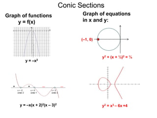
- 1. Conic Sections y2 + (x + ½)2 = ¼ (–1, 0) Graph of equations in x and y: Graph of functions y = f(x) y = –x2 y = –x(x + 2)2(x – 3)2 y2 = x3 – 6x +4
- 3. First Degree Equations Graphs of 1st degree equations Ax + By = C are straight lines.
- 4. First Degree Equations Graphs of 1st degree equations Ax + By = C are straight lines. There are two cases.
- 5. First Degree Equations Graphs of 1st degree equations Ax + By = C are straight lines. There are two cases. I. If B ≠ 0, then solving for y we obtain the format: y = mx + b, where m = slope, and (0, b) in the y-intercept.
- 6. First Degree Equations Graphs of 1st degree equations Ax + By = C are straight lines. There are two cases. I. If B ≠ 0, then solving for y we obtain the format: y = mx + b, where m = slope, and (0, b) in the y-intercept. 2x – 3y = 12
- 7. First Degree Equations Graphs of 1st degree equations Ax + By = C are straight lines. There are two cases. I. If B ≠ 0, then solving for y we obtain the format: y = mx + b, where m = slope, and (0, b) in the y-intercept. 2x – 3y = 12 y = – 4 2 x 3
- 8. First Degree Equations Graphs of 1st degree equations Ax + By = C are straight lines. There are two cases. I. If B ≠ 0, then solving for y we obtain the format: y = mx + b, where m = slope, and (0, b) in the y-intercept. (6,0) (0,–4) 2x – 3y = 12 y = – 4 2 x 3
- 9. First Degree Equations Graphs of 1st degree equations Ax + By = C are straight lines. There are two cases. I. If B ≠ 0, then solving for y we obtain the format: y = mx + b, where m = slope, and (0, b) in the y-intercept. (6,0) (0,–4) 2x – 3y = 12 y = – 4 2 x 3
- 10. First Degree Equations Graphs of 1st degree equations Ax + By = C are straight lines. There are two cases. I. If B ≠ 0, then solving for y we obtain the format: y = mx + b, where m = slope, and (0, b) in the y-intercept. (6,0) (0,–4) –3y = 12 y = –4 2x – 3y = 12 y = – 4 2 x 3
- 11. First Degree Equations Graphs of 1st degree equations Ax + By = C are straight lines. There are two cases. I. If B ≠ 0, then solving for y we obtain the format: y = mx + b, where m = slope, and (0, b) in the y-intercept. (6,0) (0,–4) –3y = 12 y = –4 2x – 3y = 12 y = – 4 2 x 3 (0,–4)
- 12. Graphs of y = mx + b: First Degree Equations Graphs of 1st degree equations Ax + By = C are straight lines. There are two cases. I. If B ≠ 0, then solving for y we obtain the format: y = mx + b, where m = slope, and (0, b) in the y-intercept. (6,0) (0,–4) –3y = 12 y = –4 2x – 3y = 12 y = – 4 2 x 3 (0,–4)
- 13. Graphs of y = mx + b: First Degree Equations Graphs of 1st degree equations Ax + By = C are straight lines. There are two cases. I. If B ≠ 0, then solving for y we obtain the format: y = mx + b, where m = slope, and (0, b) in the y-intercept. (6,0) (0,–4) –3y = 12 y = –4 2x – 3y = 12 y = – 4 2 x 3 Il. If B = 0, then the equation is of the form x = c whose graph is a vertical line. 12 – 3x = 0 (0,–4)
- 14. Graphs of y = mx + b: First Degree Equations Graphs of 1st degree equations Ax + By = C are straight lines. There are two cases. I. If B ≠ 0, then solving for y we obtain the format: y = mx + b, where m = slope, and (0, b) in the y-intercept. (6,0) (0,–4) –3y = 12 y = –4 2x – 3y = 12 y = – 4 2 x 3 Il. If B = 0, then the equation is of the form x = c whose graph is a vertical line. 12 – 3x = 0 x = 4 (0,–4)
- 15. Graphs of y = mx + b: First Degree Equations Graphs of 1st degree equations Ax + By = C are straight lines. There are two cases. I. If B ≠ 0, then solving for y we obtain the format: y = mx + b, where m = slope, and (0, b) in the y-intercept. (6,0) (0,–4) –3y = 12 y = –4 2x – 3y = 12 y = – 4 2 x 3 Il. If B = 0, then the equation is of the form x = c whose graph is a vertical line. 12 – 3x = 0 x = 4 Graphs of x = c vertical lines: (0,–4) (4,0)
- 16. Graphs of y = mx + b: First Degree Equations Graphs of 1st degree equations Ax + By = C are straight lines. There are two cases. I. If B ≠ 0, then solving for y we obtain the format: y = mx + b, where m = slope, and (0, b) in the y-intercept. (6,0) (0,–4) –3y = 12 y = –4 2x – 3y = 12 y = – 4 2 x 3 Il. If B = 0, then the equation is of the form x = c whose graph is a vertical line. 12 – 3x = 0 x = 4 Graphs of x = c vertical lines: Graphs of 2nd degree equations: Ax2 + By2 + Cx + Dy = E, (A, B, C, D, and E are numbers) are conic-sections. (0,–4) (4,0)
- 17. Conic Sections One way to study a solid is to slice it open.
- 18. Conic Sections One way to study a solid is to slice it open. The exposed area of the sliced solid is called a cross sectional area.
- 19. Conic Sections A right circular cone One way to study a solid is to slice it open. The exposed area of the sliced solid is called a cross sectional area. Conic sections are the borders of the cross sectional areas of a right circular cone as shown.
- 20. Conic Sections A right circular cone and conic sections (wikipedia “Conic Sections”) One way to study a solid is to slice it open. The exposed area of the sliced solid is called a cross sectional area. Conic sections are the borders of the cross sectional areas of a right circular cone as shown.
- 21. Conic Sections A Horizontal Section A right circular cone and conic sections (wikipedia “Conic Sections”) One way to study a solid is to slice it open. The exposed area of the sliced solid is called a cross sectional area. Conic sections are the borders of the cross sectional areas of a right circular cone as shown.
- 22. Conic Sections A Horizontal Section A right circular cone and conic sections (wikipedia “Conic Sections”) One way to study a solid is to slice it open. The exposed area of the sliced solid is called a cross sectional area. Conic sections are the borders of the cross sectional areas of a right circular cone as shown. Circles
- 23. Conic Sections A Moderately Tilted Section A right circular cone and conic sections (wikipedia “Conic Sections”) One way to study a solid is to slice it open. The exposed area of the sliced solid is called a cross sectional area. Conic sections are the borders of the cross sectional areas of a right circular cone as shown.
- 24. Conic Sections A Moderately Tilted Section A right circular cone and conic sections (wikipedia “Conic Sections”) One way to study a solid is to slice it open. The exposed area of the sliced solid is called a cross sectional area. Conic sections are the borders of the cross sectional areas of a right circular cone as shown. Ellipses
- 25. Conic Sections A Horizontal Section A Moderately Tilted Section A right circular cone and conic sections (wikipedia “Conic Sections”) One way to study a solid is to slice it open. The exposed area of the sliced solid is called a cross sectional area. Conic sections are the borders of the cross sectional areas of a right circular cone as shown. Circles and ellipses are enclosed.
- 26. Conic Sections A right circular cone and conic sections (wikipedia “Conic Sections”) A Parallel–Section One way to study a solid is to slice it open. The exposed area of the sliced solid is called a cross sectional area. Conic sections are the borders of the cross sectional areas of a right circular cone as shown.
- 27. Conic Sections A right circular cone and conic sections (wikipedia “Conic Sections”) A Parallel–Section One way to study a solid is to slice it open. The exposed area of the sliced solid is called a cross sectional area. Conic sections are the borders of the cross sectional areas of a right circular cone as shown. Parabolas
- 28. Conic Sections A right circular cone and conic sections (wikipedia “Conic Sections”) One way to study a solid is to slice it open. The exposed area of the sliced solid is called a cross sectional area. Conic sections are the borders of the cross sectional areas of a right circular cone as shown. An Cut–away Section
- 29. Conic Sections A right circular cone and conic sections (wikipedia “Conic Sections”) One way to study a solid is to slice it open. The exposed area of the sliced solid is called a cross sectional area. Conic sections are the borders of the cross sectional areas of a right circular cone as shown. An Cut–away Section Hyperbolas
- 30. Conic Sections A right circular cone and conic sections (wikipedia “Conic Sections”) An Cut–away Section One way to study a solid is to slice it open. The exposed area of the sliced solid is called a cross sectional area. Conic sections are the borders of the cross sectional areas of a right circular cone as shown. Parabolas and hyperbolas are open. A Horizontal Section A Moderately Tilted Section Circles and ellipses are enclosed. A Parallel–Section
- 31. Conic Sections Circles Ellipses Parabolas Hyperbolas We summarize the four types of conic sections here.
- 32. Conic Sections Circles Ellipses Parabolas Hyperbolas We summarize the four types of conic sections here. (Most) Graphs of 2nd equations Ax2 + By2 + Cx + Dy = E, are conic sections.
- 33. Conic Sections (Most) Graphs of 2nd equations Ax2 + By2 + Cx + Dy = E, are conic sections. The equations Ax2 + By2 + Cx + Dy = E have conic sections that are parallel to the axes, i.e. not tilted, as graphs. Circles Ellipses Parabolas Hyperbolas We summarize the four types of conic sections here.
- 34. Conic Sections (Most) Graphs of 2nd equations Ax2 + By2 + Cx + Dy = E, are conic sections. The equations Ax2 + By2 + Cx + Dy = E have conic sections that are parallel to the axes, i.e. not tilted, as graphs. Circles Ellipses Parabolas Hyperbolas We summarize the four types of conic sections here. Graphs of Ax2 + By2 + Cx + Dy = E,
- 35. Conic Sections (Most) Graphs of 2nd equations Ax2 + By2 + Cx + Dy = E, are conic sections. The equations Ax2 + By2 + Cx + Dy = E have conic sections that are parallel to the axes, i.e. not tilted, as graphs. Circles Ellipses Parabolas Hyperbolas We summarize the four types of conic sections here. Graphs of Ax2 + By2 + Cx + Dy = E,
- 36. Conic Sections (Most) Graphs of 2nd equations Ax2 + By2 + Cx + Dy = E, are conic sections. The equations Ax2 + By2 + Cx + Dy = E have conic sections that are parallel to the axes, i.e. not tilted, as graphs. In some special cases their graphs degenerate into lines or points, or nothing. Circles Ellipses Parabolas Hyperbolas We summarize the four types of conic sections here.
- 37. Conic Sections (Most) Graphs of 2nd equations Ax2 + By2 + Cx + Dy = E, are conic sections. The equations Ax2 + By2 + Cx + Dy = E have conic sections that are parallel to the axes, i.e. not tilted, as graphs. In some special cases their graphs degenerate into lines or points, or nothing. Circles Ellipses Parabolas Hyperbolas We summarize the four types of conic sections here. x2 – y2 = 0 For example, the graphs of: x + y = 0 x – y = 0
- 38. Conic Sections (Most) Graphs of 2nd equations Ax2 + By2 + Cx + Dy = E, are conic sections. The equations Ax2 + By2 + Cx + Dy = E have conic sections that are parallel to the axes, i.e. not tilted, as graphs. In some special cases their graphs degenerate into lines or points, or nothing. Circles Ellipses Parabolas Hyperbolas We summarize the four types of conic sections here. x2 – y2 = 0 For example, the graphs of: x + y = 0 x – y = 0 x2 + y2 = 0 (0,0) (0,0) is the only solution
- 39. Conic Sections (Most) Graphs of 2nd equations Ax2 + By2 + Cx + Dy = E, are conic sections. The equations Ax2 + By2 + Cx + Dy = E have conic sections that are parallel to the axes, i.e. not tilted, as graphs. In some special cases their graphs degenerate into lines or points, or nothing. Circles Ellipses Parabolas Hyperbolas We summarize the four types of conic sections here. x2 – y2 = 0 For example, the graphs of: x + y = 0 x – y = 0 x2 = –1 x2 + y2 = 0 (0,0) (0,0) is the only solution No solution no graph
- 40. Conic Sections (Most) Graphs of 2nd equations Ax2 + By2 + Cx + Dy = E, are conic sections. The equations Ax2 + By2 + Cx + Dy = E have conic sections that are parallel to the axes, i.e. not tilted, as graphs. In some special cases their graphs degenerate into lines or points, or nothing. We will match these 2nd degree equations with different conic sections using the algebraic method "completing the square". Circles Ellipses Parabolas Hyperbolas We summarize the four types of conic sections here.
- 41. Conic Sections (Most) Graphs of 2nd equations Ax2 + By2 + Cx + Dy = E, are conic sections. The equations Ax2 + By2 + Cx + Dy = E have conic sections that are parallel to the axes, i.e. not tilted, as graphs. In some special cases their graphs degenerate into lines or points, or nothing. We will match these 2nd degree equations with different conic sections using the algebraic method "completing the square". “Completing the Square“ is THE main algebraic algorithm for handling all 2nd degree formulas. Circles Ellipses Parabolas Hyperbolas We summarize the four types of conic sections here.
- 42. Conic Sections (Most) Graphs of 2nd equations Ax2 + By2 + Cx + Dy = E, are conic sections. The equations Ax2 + By2 + Cx + Dy = E have conic sections that are parallel to the axes, i.e. not tilted, as graphs. In some special cases their graphs degenerate into lines or points, or nothing. We will match these 2nd degree equations with different conic sections using the algebraic method "completing the square". “Completing the Square“ is THE main algebraic algorithm for handling all 2nd degree formulas. We need the Distance Formula D = Δx2 + Δy2 for the geometry. Circles Ellipses Parabolas Hyperbolas We summarize the four types of conic sections here.
- 43. Circles A circle is the set of all the points that have equal distance r, called the radius, to a fixed point C which is called the center.
- 44. Circles A circle is the set of all the points that have equal distance r, called the radius, to a fixed point C which is called the center. C
- 45. r r Circles A circle is the set of all the points that have equal distance r, called the radius, to a fixed point C which is called the center. C
- 46. r r Circles A circle is the set of all the points that have equal distance r, called the radius, to a fixed point C which is called the center. C
- 47. r r The radius and the center completely determine the circle. Circles A circle is the set of all the points that have equal distance r, called the radius, to a fixed point C which is called the center. C
- 48. r The radius and the center completely determine the circle. Circles Let (h, k) be the center of a circle and r be the radius. (h, k) A circle is the set of all the points that have equal distance r, called the radius, to a fixed point C which is called the center. r C
- 49. r The radius and the center completely determine the circle. Circles (x, y) Let (h, k) be the center of a circle and r be the radius. Suppose (x, y) is a point on the circle, then the distance between (x, y) and the center is r. (h, k) A circle is the set of all the points that have equal distance r, called the radius, to a fixed point C which is called the center. r C
- 50. r The radius and the center completely determine the circle. Circles (x, y) Let (h, k) be the center of a circle and r be the radius. Suppose (x, y) is a point on the circle, then the distance between (x, y) and the center is r. Hence, (h, k) r = (x – h)2 + (y – k)2 A circle is the set of all the points that have equal distance r, called the radius, to a fixed point C which is called the center. r C
- 51. r The radius and the center completely determine the circle. Circles (x, y) Let (h, k) be the center of a circle and r be the radius. Suppose (x, y) is a point on the circle, then the distance between (x, y) and the center is r. Hence, (h, k) r = (x – h)2 + (y – k)2 or r2 = (x – h)2 + (y – k)2 A circle is the set of all the points that have equal distance r, called the radius, to a fixed point C which is called the center. r C
- 52. r The radius and the center completely determine the circle. Circles (x, y) Let (h, k) be the center of a circle and r be the radius. Suppose (x, y) is a point on the circle, then the distance between (x, y) and the center is r. Hence, (h, k) r = (x – h)2 + (y – k)2 or r2 = (x – h)2 + (y – k)2 This is called the standard form of circles. A circle is the set of all the points that have equal distance r, called the radius, to a fixed point C which is called the center. r C
- 53. r The radius and the center completely determine the circle. Circles (x, y) Let (h, k) be the center of a circle and r be the radius. Suppose (x, y) is a point on the circle, then the distance between (x, y) and the center is r. Hence, (h, k) r = (x – h)2 + (y – k)2 or r2 = (x – h)2 + (y – k)2 This is called the standard form of circles. Given an equation of this form, we can easily identify the center and the radius. A circle is the set of all the points that have equal distance r, called the radius, to a fixed point C which is called the center. r C
- 54. r2 = (x – h)2 + (y – k)2 Circles
- 55. r2 = (x – h)2 + (y – k)2 must be “ – ” Circles
- 56. r2 = (x – h)2 + (y – k)2 r is the radius must be “ – ” Circles
- 57. r2 = (x – h)2 + (y – k)2 r is the radius must be “ – ” (h, k) is the center Circles
- 58. r2 = (x – h)2 + (y – k)2 r is the radius must be “ – ” (h, k) is the center Circles Example B. Write the equation of the circle as shown. (–1, 3)
- 59. r2 = (x – h)2 + (y – k)2 r is the radius must be “ – ” (h, k) is the center Circles Example B. Write the equation of the circle as shown. The center is (–1, 3) and the radius is 5. (–1, 3)
- 60. r2 = (x – h)2 + (y – k)2 r is the radius must be “ – ” (h, k) is the center Circles Example B. Write the equation of the circle as shown. The center is (–1, 3) and the radius is 5. Hence the equation is: 52 = (x – (–1))2 + (y – 3)2 (–1, 3)
- 61. r2 = (x – h)2 + (y – k)2 r is the radius must be “ – ” (h, k) is the center Circles Example B. Write the equation of the circle as shown. The center is (–1, 3) and the radius is 5. Hence the equation is: 52 = (x – (–1))2 + (y – 3)2 or 25 = (x + 1)2 + (y – 3 )2 (–1, 3)
- 62. Example C. Identify the center and the radius of 16 = (x – 3)2 + (y + 2)2. Label the top, bottom, left and right most points. Graph it. Circles
- 63. Example C. Identify the center and the radius of 16 = (x – 3)2 + (y + 2)2. Label the top, bottom, left and right most points. Graph it. Put 16 = (x – 3)2 + (y + 2)2 into the standard form: 42 = (x – 3)2 + (y – (–2))2 Circles
- 64. Example C. Identify the center and the radius of 16 = (x – 3)2 + (y + 2)2. Label the top, bottom, left and right most points. Graph it. Put 16 = (x – 3)2 + (y + 2)2 into the standard form: 42 = (x – 3)2 + (y – (–2))2 Hence r = 4, center = (3, –2) Circles
- 65. Example C. Identify the center and the radius of 16 = (x – 3)2 + (y + 2)2. Label the top, bottom, left and right most points. Graph it. Put 16 = (x – 3)2 + (y + 2)2 into the standard form: 42 = (x – 3)2 + (y – (–2))2 Hence r = 4, center = (3, –2) (3,–2) Circles r = 4
- 66. Example C. Identify the center and the radius of 16 = (x – 3)2 + (y + 2)2. Label the top, bottom, left and right most points. Graph it. Put 16 = (x – 3)2 + (y + 2)2 into the standard form: 42 = (x – 3)2 + (y – (–2))2 Hence r = 4, center = (3, –2) (3,–2) Circles r = 4
- 67. Example C. Identify the center and the radius of 16 = (x – 3)2 + (y + 2)2. Label the top, bottom, left and right most points. Graph it. Put 16 = (x – 3)2 + (y + 2)2 into the standard form: 42 = (x – 3)2 + (y – (–2))2 Hence r = 4, center = (3, –2) (3,–2) Circles When equations are not in the standard form, we have to rearrange them into the standard form. We do this by "completing the square". r = 4
- 68. Example C. Identify the center and the radius of 16 = (x – 3)2 + (y + 2)2. Label the top, bottom, left and right most points. Graph it. Put 16 = (x – 3)2 + (y + 2)2 into the standard form: 42 = (x – 3)2 + (y – (–2))2 Hence r = 4, center = (3, –2) (3,–2) Circles When equations are not in the standard form, we have to rearrange them into the standard form. We do this by "completing the square". To complete the square means to add a number to an expression so the sum is a perfect square. r = 4
- 69. Example C. Identify the center and the radius of 16 = (x – 3)2 + (y + 2)2. Label the top, bottom, left and right most points. Graph it. Put 16 = (x – 3)2 + (y + 2)2 into the standard form: 42 = (x – 3)2 + (y – (–2))2 Hence r = 4, center = (3, –2) (3,–2) Circles When equations are not in the standard form, we have to rearrange them into the standard form. We do this by "completing the square". To complete the square means to add a number to an expression so the sum is a perfect square. This procedure is the main technique in dealing with 2nd degree equations. r = 4
- 71. (Completing the Square) Circles Example D. Fill in the blank to make a perfect square. a. x2 – 6x + (–6/2)2 = x2 – 6x + 9 = (x – 3)2 b. y2 + 12y + (12/2)2 = y2 + 12y + 36 = ( y + 6)2
- 72. (Completing the Square) If we are given x2 + bx, then adding (b/2)2 to the expression makes the expression a perfect square, Circles Example D. Fill in the blank to make a perfect square. a. x2 – 6x + (–6/2)2 = x2 – 6x + 9 = (x – 3)2 b. y2 + 12y + (12/2)2 = y2 + 12y + 36 = ( y + 6)2
- 73. (Completing the Square) If we are given x2 + bx, then adding (b/2)2 to the expression makes the expression a perfect square, Circles Example D. Fill in the blank to make a perfect square. a. x2 – 6x + (–6/2)2 b. y2 + 12y + (12/2)2 = y2 + 12y + 36 = ( y + 6)2
- 74. (Completing the Square) If we are given x2 + bx, then adding (b/2)2 to the expression makes the expression a perfect square, Circles Example D. Fill in the blank to make a perfect square. a. x2 – 6x + (–6/2)2 = x2 – 6x + 9 = (x – 3)2 b. y2 + 12y + (12/2)2 = y2 + 12y + 36 = ( y + 6)2
- 75. (Completing the Square) If we are given x2 + bx, then adding (b/2)2 to the expression makes the expression a perfect square, i.e. x2 + bx + (b/2)2 is the perfect square (x + b/2)2. Circles Example D. Fill in the blank to make a perfect square. a. x2 – 6x + (–6/2)2 = x2 – 6x + 9 = (x – 3)2 b. y2 + 12y + (12/2)2 = y2 + 12y + 36 = ( y + 6)2
- 76. (Completing the Square) If we are given x2 + bx, then adding (b/2)2 to the expression makes the expression a perfect square, i.e. x2 + bx + (b/2)2 is the perfect square (x + b/2)2. Circles Example D. Fill in the blank to make a perfect square. a. x2 – 6x + (–6/2)2 = x2 – 6x + 9 = (x – 3)2 b. y2 + 12y + (12/2)2
- 77. (Completing the Square) If we are given x2 + bx, then adding (b/2)2 to the expression makes the expression a perfect square, i.e. x2 + bx + (b/2)2 is the perfect square (x + b/2)2. Circles Example D. Fill in the blank to make a perfect square. a. x2 – 6x + (–6/2)2 = x2 – 6x + 9 = (x – 3)2 b. y2 + 12y + (12/2)2
- 78. (Completing the Square) If we are given x2 + bx, then adding (b/2)2 to the expression makes the expression a perfect square, i.e. x2 + bx + (b/2)2 is the perfect square (x + b/2)2. Circles Example D. Fill in the blank to make a perfect square. a. x2 – 6x + (–6/2)2 = x2 – 6x + 9 = (x – 3)2 b. y2 + 12y + (12/2)2 = y2 + 12y + 36
- 79. (Completing the Square) If we are given x2 + bx, then adding (b/2)2 to the expression makes the expression a perfect square, i.e. x2 + bx + (b/2)2 is the perfect square (x + b/2)2. Circles Example D. Fill in the blank to make a perfect square. a. x2 – 6x + (–6/2)2 = x2 – 6x + 9 = (x – 3)2 b. y2 + 12y + (12/2)2 = y2 + 12y + 36 = ( y + 6)2
- 80. (Completing the Square) If we are given x2 + bx, then adding (b/2)2 to the expression makes the expression a perfect square, i.e. x2 + bx + (b/2)2 is the perfect square (x + b/2)2. Circles Example D. Fill in the blank to make a perfect square. a. x2 – 6x + (–6/2)2 = x2 – 6x + 9 = (x – 3)2 b. y2 + 12y + (12/2)2 = y2 + 12y + 36 = ( y + 6)2 The following are the steps in putting a 2nd degree equation into the standard form.
- 81. (Completing the Square) If we are given x2 + bx, then adding (b/2)2 to the expression makes the expression a perfect square, i.e. x2 + bx + (b/2)2 is the perfect square (x + b/2)2. Circles Example D. Fill in the blank to make a perfect square. a. x2 – 6x + (–6/2)2 = x2 – 6x + 9 = (x – 3)2 b. y2 + 12y + (12/2)2 = y2 + 12y + 36 = ( y + 6)2 The following are the steps in putting a 2nd degree equation into the standard form. 1. Group the x2 and the x–terms together, group the y2 and y terms together, and move the number term the the other side of the equation.
- 82. (Completing the Square) If we are given x2 + bx, then adding (b/2)2 to the expression makes the expression a perfect square, i.e. x2 + bx + (b/2)2 is the perfect square (x + b/2)2. Circles Example D. Fill in the blank to make a perfect square. a. x2 – 6x + (–6/2)2 = x2 – 6x + 9 = (x – 3)2 b. y2 + 12y + (12/2)2 = y2 + 12y + 36 = ( y + 6)2 The following are the steps in putting a 2nd degree equation into the standard form. 1. Group the x2 and the x–terms together, group the y2 and y terms together, and move the number term the the other side of the equation. 2. Complete the square for the x–terms and for the y–terms. Make sure you add the necessary numbers to both sides.
- 83. Example E. Use completing the square to find the center and radius of x2 – 6x + y2 + 12y = –36. Find the top, bottom, left and right most points. Graph it. Circles
- 84. Example E. Use completing the square to find the center and radius of x2 – 6x + y2 + 12y = –36. Find the top, bottom, left and right most points. Graph it. We use completing the square to put the equation into the standard form: Circles
- 85. Example E. Use completing the square to find the center and radius of x2 – 6x + y2 + 12y = –36. Find the top, bottom, left and right most points. Graph it. We use completing the square to put the equation into the standard form: x2 – 6x + + y2 + 12y + = –36 Circles
- 86. Example E. Use completing the square to find the center and radius of x2 – 6x + y2 + 12y = –36. Find the top, bottom, left and right most points. Graph it. We use completing the square to put the equation into the standard form: x2 – 6x + + y2 + 12y + = –36 ;complete squares x2 – 6x + 9 + y2 + 12y + 36 = –36 + 9 + 36 Circles
- 87. Example E. Use completing the square to find the center and radius of x2 – 6x + y2 + 12y = –36. Find the top, bottom, left and right most points. Graph it. We use completing the square to put the equation into the standard form: x2 – 6x + + y2 + 12y + = –36 ;complete squares x2 – 6x + 9 + y2 + 12y + 36 = –36 + 9 + 36 Circles
- 88. Example E. Use completing the square to find the center and radius of x2 – 6x + y2 + 12y = –36. Find the top, bottom, left and right most points. Graph it. We use completing the square to put the equation into the standard form: x2 – 6x + + y2 + 12y + = –36 ;complete squares x2 – 6x + 9 + y2 + 12y + 36 = –36 + 9 + 36 ( x – 3 )2 + (y + 6)2 = 9 Circles
- 89. Example E. Use completing the square to find the center and radius of x2 – 6x + y2 + 12y = –36. Find the top, bottom, left and right most points. Graph it. We use completing the square to put the equation into the standard form: x2 – 6x + + y2 + 12y + = –36 ;complete squares x2 – 6x + 9 + y2 + 12y + 36 = –36 + 9 + 36 ( x – 3 )2 + (y + 6)2 = 9 ( x – 3 )2 + (y + 6)2 = 32 Circles
- 90. Example E. Use completing the square to find the center and radius of x2 – 6x + y2 + 12y = –36. Find the top, bottom, left and right most points. Graph it. We use completing the square to put the equation into the standard form: x2 – 6x + + y2 + 12y + = –36 ;complete squares x2 – 6x + 9 + y2 + 12y + 36 = –36 + 9 + 36 ( x – 3 )2 + (y + 6)2 = 9 ( x – 3 )2 + (y + 6)2 = 32 Hence the center is (3 , –6), and radius is 3. Circles
- 91. Example E. Use completing the square to find the center and radius of x2 – 6x + y2 + 12y = –36. Find the top, bottom, left and right most points. Graph it. We use completing the square to put the equation into the standard form: x2 – 6x + + y2 + 12y + = –36 ;complete squares x2 – 6x + 9 + y2 + 12y + 36 = –36 + 9 + 36 ( x – 3 )2 + (y + 6)2 = 9 ( x – 3 )2 + (y + 6)2 = 32 Hence the center is (3 , –6), and radius is 3. Circles
- 92. Example E. Use completing the square to find the center and radius of x2 – 6x + y2 + 12y = –36. Find the top, bottom, left and right most points. Graph it. We use completing the square to put the equation into the standard form: x2 – 6x + + y2 + 12y + = –36 ;complete squares x2 – 6x + 9 + y2 + 12y + 36 = –36 + 9 + 36 ( x – 3 )2 + (y + 6)2 = 9 ( x – 3 )2 + (y + 6)2 = 32 Hence the center is (3 , –6), and radius is 3. Circles
- 93. Example E. Use completing the square to find the center and radius of x2 – 6x + y2 + 12y = –36. Find the top, bottom, left and right most points. Graph it. We use completing the square to put the equation into the standard form: x2 – 6x + + y2 + 12y + = –36 ;complete squares x2 – 6x + 9 + y2 + 12y + 36 = –36 + 9 + 36 ( x – 3 )2 + (y + 6)2 = 9 ( x – 3 )2 + (y + 6)2 = 32 Hence the center is (3 , –6), and radius is 3. Circles (3 ,–9) (3 , –3) (0 ,–6) (6 ,–6)
- 94. Conic Sections
- 95. Circles B. Find the radius and the center of each circle. Draw and label the four cardinal points. 1 = x 2 + y 2 1. 4 = x 2 + y 2 2. 1 = (x – 1)2 + (y – 3 )2 4. 4 = (x + 1)2 + (y + 5)2 5. 1/9 = x2 + y2 3. 1/4 = (x – 2)2 + (y + 3/2)2 6. 16 = (x + 5)2 + (y – 3)2 7. 25 = (x + 5)2 + (y – 4)2 8. 9 = (x + 1)2 + (y + 3)2 9. 1/16 = (x – 4)2 + (y – 6)2 10. 9/16 = (x + 7)2 + (y – 8)2 11. 1/100 = (x + 1.2)2 + (y – 4.1)2 12. 9/49 = (x + 9)2 + (y + 8)2 13. 0.01 = (x – 1.5 )2 + (y + 3.5)2 14. 0.49 = (x + 3.5)2 + (y + 0.5)2 15.
- 96. 2. C. Complete the square to find the center and radius of each of the following circles. Draw and label the four cardinal points. 1. 4. 3. 6. 5. 8. 7. 13. 14. Approximate the radius In the following problems. x2 + y2 – 2y = 35 x2 – 8x + y2 + 12y = 92 x2 – 4y + y2 + 6x = –4 y2 – 8x + x2 + 2y = 8 x2 + 18y + y2 – 8x = 3 2x2 – 8x + 2y2 +12y = 1 x2 – 6x + y2 + 12y = –9 x2 + y2 + 8y = –7 x2 + 4x + y2 = 96 Circles x2 + 6y + y2 – 16x = –9 10. 9. x2 – x + y2 + 3y = 3/2 x2 + 3y + y2 – 5x = 1/2 12. 11. x2 – 0.4x + y2 + 0.2y = 0.3 x2 + 0.8y + y2 – 1.1x = –0.04
- 97. 1. The circle that has (3,1) and (1,3) as its diameter. D. Use the midpoint formula and the distance formula to find the center and the radius of each circle. Then find the equation of each circle. Circles 2. The circle that has (–2,4) and (0,–3) as its diameter. 3. 4. The circle that has (6, –3) and (0,–3) as its diameter. The circle that has (5,–4) and (–2,–1) as its diameter.
- 98. (Answers to odd problems) Ex. A 1. x2 + y2 = 25 5. (x – 1)2 + y2 = 9 3. x2 + y2 = 5 7. (x – 1)2 + (y + 1)2 = 81 9. (x + 3)2 + (y + 2)2 = 16 Circles (0,5) (0,-5) (5,0) (-5,0) (0,√5) (0,-√5) (√5,0) (-√5,0) (1,3) (1,-3) (4,0) (-2,0) (1,8) (1,-10) (10,0) (-8,0) (-3,2) (-3,-6) (1,-2) (-2,-2)
- 99. Exercise B. 1. C = (0,0), r = 1. 5. C = (-1,-5), r = 2. 3. C = (0,0), r = 1/3. 7. C = (-5,3), r = 4. 9. C = (-1,-3), r = 3. 11. C = (-7,8), r = ¾. Circles (0,1) (0,-1) (1,0) (-1,0) (0,1/3) (0,-1/3) (1/3,0) (-1/3,0) (-1,-3) (-1,-7) (1,-5) (-3,-5) (-5,7) (-5,-1) (-1,3) (-9,3) (-1,0) (-1,-6) (2,-3) (-4,-3) (-7,8.75) (-7,7.25) (-6.25,8) (-7.75,8)
- 100. 13. C = (-9,-8), r = 3/7. 15. C = (-3.5,-0.5), r = 0.7. Exercise C. 5. C = (-3,2), r = 3. 3. C = (0,-4), r = 3. 1. C = (-2,0), r = 10. Circles (-9,-53/7) (-9,-59/7) (-60/7,-8) (-66/7,-8) (-3.5,0.2) (-3.5,-1.2) (-2.8,-0.5) (-4.2,-0.5) (-2,10) (-2,-10) (8,0) (-12,0) (0,-1) (0,-7) (3,-4) (-3,-4) (-3,5) (-3,-1) (0,2) (-6,2)
- 101. 7. C = (4,-6), r = 12. 9. C = (1/2,-3/2), r = 2. 13. C = (0.2,-0.1), r = 0.5916 11. C = (3, -6), r = 6. Circles (3,0) (3,-12) (8,-6) (-2,-6) (1/2,1/2) (1/2,-7/2) (5/2,-3/2) (-3/2,-3/2) (4,6) (4,-18) (16,-6) (-8,-6)
- 102. 1. C = (2, 2), r = √2. Equation: (x – 2)2 + (y – 2)2 = 2 Exercise D. 3. C = (3/2, -5/2), r = (√58)/2. Equation: (x – 3/2)2 + (y + 5/2)2 = 14.5 Circles