control design

1. 1
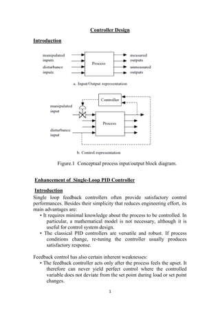
Controller Design
Introduction
Figure.1 Conceptual process input/output block diagram.
Enhancement of Single-Loop PID Controller
Introduction
Single loop feedback controllers often provide satisfactory control
performances. Besides their simplicity that reduces engineering effort, its
main advantages are:
• It requires minimal knowledge about the process to be controlled. In
particular, a mathematical model is not necessary, although it is
useful for control system design.
• The classical PID controllers are versatile and robust. If process
conditions change, re-tuning the controller usually produces
satisfactory response.
Feedback control has also certain inherent weaknesses:
• The feedback controller acts only after the process feels the upset. It
therefore can never yield perfect control where the controlled
variable does not deviate from the set point during load or set point
changes.

2. 2
• Poor feedback tuning may cause instability
• PID controller does not always provide the best possible control for
all processes especially for processes with large dead times and/or
cascade processes with large time constant.
• In some applications the controlled variable cannot be measured on
line and consequently feedback control is not feasible.
• Feedback control does not provide predictive control action to
compensate for the effects of known or measurable disturbances.
Possible configurations that improves the feedback controller design by
taking advantage of additional knowledge about process dynamics
through one of these means:
 Additional process output measurements are used (e.g. cascade
,inferential)
• Additional process inputs measurements are used (e.g. feed-forward)
• Use explicit modeling in control calculations (e.g. inferential)
• Use a different control algorithm than PID (e.g. feed-forward)
Cascade Control
In a cascade control configuration we have one manipulated variable
and two measurements.
Example (1)
Consider the stirred tank heater of Figure 1 for which the objective is to
control the exit temperature, T using the heating oil flow, Fc
.
Conventional control
Uses a single feedback loop with T as CV and Fc
as MV.
Conventional control: uses a single feedback loop with T as CV and Fc
as
MV.

3. 3
Figure 2: Stirred Tank Heater with single control loop
Figure 3: Dynamic response of stirred tank heater to disturbance in oil
pressure using single loop controller

4. 4
1. Cascade control
Uses a secondary measured process input which is the heating oil flow
because it responds faster to the disturbances in the oil pressure.
Figure 4: Stirred Tank heater with cascade control
Figure 5: Dynamic response of stirred tank heater to disturbance in oil
pressure with cascade control
We notice:
• We can have two control loops using two different measurements
(T, Fc
), but sharing a common manipulated variable.

5. 5
• The loop that measures T is the primary or master, or outer loop
and uses a set point supplied by the user.
• The loop that measures Fc
uses the output of the primary loop as its
set point and is called the secondary, or slave, or inner loop.
The block diagram for the conventional control is shown in Figure 6 and
that for cascade control is shown in Figure 7.
Figure 6: Block diagram of Conventional controller
Figure 7: Cascade control block diagram
Advantages
The advantages of cascade control can be summarized as follow:
• Disturbances felt by the secondary variable, is significantly corrected
by the secondary controller before it is felt by the process.
• The dynamics of the secondary loop are much faster than those of
the primary loop. This allows the use of higher gains in the
secondary controller to suppress more effectively the effect of the
disturbance occurring in the secondary loop without affecting the
stability of the system.
Selection of the secondary variable
The key point in cascade control is the selection of secondary variable:
• The secondary variable must indicate the occurrence of an important
disturbance
• The secondary variable dynamics must be faster that the primary
variable dynamics
Implementation issues
Cascade controller modes and tuning:

6. 6
• The secondary loop is normally P or PI controller. Derivative modes
are not advised in the secondary loop. The primary loop is usually
PI or PID controller.
• The cascade controller is tuned in a sequential manner. The
secondary controller is first tuned satisfactorily and the primary is
then tuned.
Cascade controller is desired when:
• Single loop does not provide satisfactory performance
• A measured secondary variable is available
• The secondary loop should be three times as fast as the primary.
2. Selective (override) control (MV<CV)
If a process has fewer manipulated variables than controlled variables, a
strategy is needed for sharing the manipulated variables among the
controlled variables. A common strategy is to use selectors to choose the
appropriate process variables among a number of available
measurements.
2.1 Maintaining Safety of the Equipment
Examples of these situations include:
• Safeguard the operation of variable speed pumps.
• Safeguard the operation of high temperature or pressure reactors.
• Avoid flooding in distillation columns
• Safeguard the operation of furnace.
The selector compares signals P1
and P2
and chooses the highest one. This
type of control is also called override control.
If q < qmin
: switch from level control to Flow control
2.2 Improving Control Performance
Plug flow reactor with moving hot spot. A control strategy that
accomplishes this goal is shown in Fig 9. The high selector selects the
transmitter with the highest output and the control is based on this
temperature.

7. 7
Figure 8: A selective control for sand-water slurry system
Figure 9: A plug flow reactor with selective control
2.3 Optimization of the process
Consider the furnace of Figure 10, where fuel oil is used to provide heat
to a number of process units. Each individual unit manipulates the flow of
oil required to maintain its controlled variable at set point. A bypass
control loop is also provided. A bad or inefficient operation of the process
is the one for which the oil temperature is heated above the value that
would satisfy the need of the users. In this case most of the valves would
not be wide open and large quantity of fuel would be burned to reach the
unnecessary high oil temperature. The effective operation that would save
energy is the one that would maintain the oil leaving the furnace at a
temperature just enough to provide the necessary energy to the users with
hardly any flow through the bypass valve. In this case most of the
temperature control valves would be open most of the time. To achieve
this goal, the selective control strategy, shown in Figure 10, first selects

8. 8
the most open valve using a high selector. The valve position controller
controls the selected valve position at large value i.e. 90 % open by
manipulating the set point of the furnace temperature. This saves energy
because it will maintain the temperature just hot enough to provide
needed heat to the users.
Figure 10: Hot oil system
2.4 Protecting against sensor/transmitters failures
Selectors are also used to protect against transmitter failures by
selecting a valid transmitter signal among several. Redundant transmitters
monitor the process variable and the median selector chooses the right
one for control. Redundant sensors are commonly used in a hostile
environment of high temperature or corrosive where failures rate are high
thus avoiding the shutdown of the process.
2.5 Other Override Control examples
• Protection of Boiler system
• Protecting a compressor system

9. 9
Figure 11: Boiler
Figure 12: Compressor System
3. Split Range Control (MV > CV)
This control configuration has one controlled variable and more than one
manipulated variable.
A single process output is controlled by coordinating the actions of
several manipulated variables.
Remarks:
• This type of control configuration is not very common in chemical
industry.
• The error signal is split into several parts, either equally or at
specified ratio, to regulate several manipulated variables.

10. 11
Figure 13: Example of Split Range Control
4. Ratio Control
In some aspects ratio control can be considered as a special type of feed-
forward control where two loads are measured and held in a constant ratio
to each other.

11. 11
Figure 14: Ratio Control Example
4.1 Applications of Ratio Control
Ratio control is used for a variety of applications including:
• Keep constant the ratio between the feed flow rate and the steam in
the reboiler of a distillation column,
• Hold constant the reflux ratio in a distillation column.
• Control the ratio of two reactants entering a reactor at a desired
value.
• Hold the ratio of two blended streams constant in order to maintain
the composition of the blend at the desired value.
• Hold the ratio of a purge stream to the recycle stream constant.
• Keep the ratio of fuel/air in a burner at its optimum value
• Maintain the ratio of the liquid flow rate to vapor flow rate in an
absorption column constant.

12. 12
Figure 15: Examples of Ratio Control
5. Inferential Control
In some case, the controlled variable can not be measured directly or
continuously such as
• Reid Vapor pressure
• Density
• Melt Index
• Molecular weight
• Gas composition
Therefore, inferential control makes use of a secondary measurement to
estimate (infer) the unmeasured variable.
Inferring the unmeasured output can be achieved through:
• Using physical laws, (Relating T to C through thermodynamic)
• Using a model equation

13. 13
• Using Empirical modeling
5.1 Inferential control through modeling
Consider the block diagram of the process shown in Fig 16, with one
unmeasured controlled output y and one secondary measured output z.
Figure 16: Process with need for inferential control
The open loop transfer function:
We can solve for d(s) in the second equation to find the following
estimate of the unmeasured disturbance
)
3
(
)
(
)
(
2
)
(
2
)
(
)
(
2
1
)
( s
u
s
d
G
s
p
G
s
z
s
d
G
s
d 

Substituting back in equation (1) yields,
This equation provides the estimator needed which relates the
unmeasured controlled output to measured variables u(s) and z(s). Figure
17 shows the resulting block diagram for the inferential control.

14. 14
Figure 17: Process under inferential control system
Remarks:
• Generally inferential control is used when composition is the desired
controlled variable. Temperature is the most common secondary
measurement.
• From Equation (4), the accuracy of the inferential control scheme
depends on the good estimation, e.g. depends on the good knowledge of
the process Gp1
(s), Gp2
(s), Gd1
(s) and Gd2
(s). Generally these process
elements are not known perfectly and therefore the inferential control
would provide control with varying quality.
Example (2): Inferential control of a distillation column
Consider a distillation column, which separates a mixture of propane-
butane in two products. The reflux ratio is the manipulated variable. The
feed and overhead compositions are unmeasured so there is need for
inferential control. The secondary measurement to infer the overhead
composition is the temperature at the top tray. The process inputs are the
feed composition (disturbance) and reflux ratio (manipulated variable)
while the outputs are the overhead propane composition (unmeasured
controlled variable) and temperature of top tray (secondary
measurement).

15. 15
Figure 18: (a) Block diagram of distillation column; (b) corresponding
inferential
5.2 Nonlinear (Empirical) Inferential systems
Recently, online estimation techniques such neural networks have been
used to estimate unmeasured variables from available plant data. The
output estimator is called soft sensor.
Empirical inferential system is not limited to the use of NN. Any linear
regression methods can be used to correlate the unmeasured variable to
the measurements of secondary variable or other measured process
variables.
5.3 Implementation issues
Inferential control is appropriate when:
• Measurement of the true controlled variable is not available because:

16. 16
 An on-stream sensor is not possible
 An on-stream sensor is too costly
 Sensor has unfavorable dynamics (long time delay, lab
analysis)
 A measured inferential variable is available.
6. Feed Forward Control
Feed forward control attempts to enhance the performance of the single
loop feedback control by making use of an additional measurement of
process input as shown in Figure 19.
Figure 19: Feed Forward Block diagram
In the feed forward, the disturbance is measured directly and the
manipulated variable is changed accordingly to eliminate the impact of
the disturbance on process output. While the feedback controller reacts
only after it has detected a deviation of the value of the output from the
desired steady state.
Example (2)
Consider the example of the stirred tank heater of Figure 20. The
objective is to control the temperature. The disturbance source is Ti
.
Note:
Feed forward can be developed for more than one disturbance. The
controller acts according to which disturbance is active. Fro example, we
can measure both Ti
and Fi
.

17. 17
Figure 20a: Feedback control of heated storage tank
Figure 20b: Feed Forward control of Heated storage tank
FF Controller design example
Consider the heated storage tank, the modeling equation is:
The heat load, Q can be related to the steam temperature or pressure, or to
the latent heat:
Steady state design
At steady state, dT/dt = 0, therefore:

18. 18
Therefore in order to keep the controlled variable, i.e. temperature T at
the set point T
sp
, the manipulated variable, i.e. amount of steam should
be:
Figure 21: Steady-state Feed Forward controller design
Remarks:
• SS FFC requires minimum calculations and a detailed model is not
required.
• SS FFC may not perform well during transient conditions because
the dynamic is ignored.
Dynamic design
The dynamic equation of the heated tank can be written as:

19. 19
Figure 22: Dynamic Feed Forward controller design
6.1 Disadvantages
• The disturbances are not always measured.
• The quality o f FFC depends on the accuracy of the model.
• FFC design may lead to unrealizable control systems.
6.2 General FFC Design
Consider the block diagram for the open-loop systems shown in Figure
23. It is clear that:

20. 21
Figure 23: Open-loop process
Let y
sp
be the desired set point for the controlled variable:
u(s) is the output of the feed-forward controller . Therefore, the block
diagram with FFC looks:
Applying this control law to the heated tank example:

21. 21
The block diagram including measurement device and final control
element becomes:
From the block diagram we can write the overall transfer function:
Disturbance rejection: in that case y = y
sp
= 0, therefore, the last design
equation gives:
Set point tracking: in that case, y = y
sp
and d = 0, therefore, the design
equation ends up as:

22. 22
Figure 24: Process under feed forward control
6.3 Simplification of FFC design
In the absence of exact representation of the model, the FFC can be
approximated by the following:
Where α and β are design parameters.
Note: If Gp
or Gd
has time delay, then the resulting FF controller is
unrealizable.
Nevertheless, Feedback is still necessary for set point tracking, rejecting
other unmeasured disturbance, correcting for model uncertainty.
Feed-Forward should be used when:
• Feedback control does not provide satisfactory performance.
• A measured feed-forward variable is available.

23. 23
6.4 Conclusions
Advantages disadvantages
Feed-Forward
1. acts before the effect of a
disturbance has been felt by the
system
2. Is good for slow systems
3. It does not introduce instability
in the closed-loop response
1. Requires identification of all
possible disturbances and their
measurement.
2. Can not cope with unmeasured
disturbances.
3. Sensitive to process parameter
variation.
4. Require good knowledge of the
process model
Feedback
1. Does not require
identification of all possible
disturbances and their
measurement.
2. It is insensitive to modeling
error.
3. It is insensitive to parameter
changes.
1. It waits until the effect of
disturbance is felt by the system.
2. It is unsatisfactory for slow
systems.
3. It may create instability in the
closed-loop response.
7. Feed-Forward plus Feedback Control
To combine the advantages of both Feed-forward and feedback
controllers, one can consider the hybrid control system with Gm
= Gv
=1,

24. 24
Figure 25: Feedback + Feed-Forward Control system
We notice:
1. The stability of the overall system is still given by the same
characteristic equation.
The stability characteristic of a feedback system is not
affected by the addition of a feed-forward loop.
2. The feed-forward controller is still given by the same law as before.
Applying the hybrid FF and Feedback control system for the heated tank
is shown in the Figure 26:
We notice:
Offset may occur when FF alone is used with some modeling error occurs
in the steady state gain of the FF controller.
Remark:

25. 25
If the dynamic of the disturbance is faster than that of the manipulated
variable, i.e. τd
<τp
, then using Hybrid FF and FB leads to double
correction, which may cause large overshoot and poor performance.
Figure 26: Hybrid Feed-Forward and Feedback control of Heated Tank
Figure 27: Comparison between FF and FF+FB control systems