This document provides an overview of common feedback control modes including proportional (P), integral (I), derivative (D), and PID control. It defines the basic control equations for each mode and discusses their transfer functions. P control reduces error proportionally but can result in steady-state offset. I control eliminates offset by integrating the error over time. D control anticipates changes in error to improve response. PID combines all three for the best performance but is most complex to tune. The document also covers practical considerations like controller forms, manual vs automatic modes, and derivative filtering.

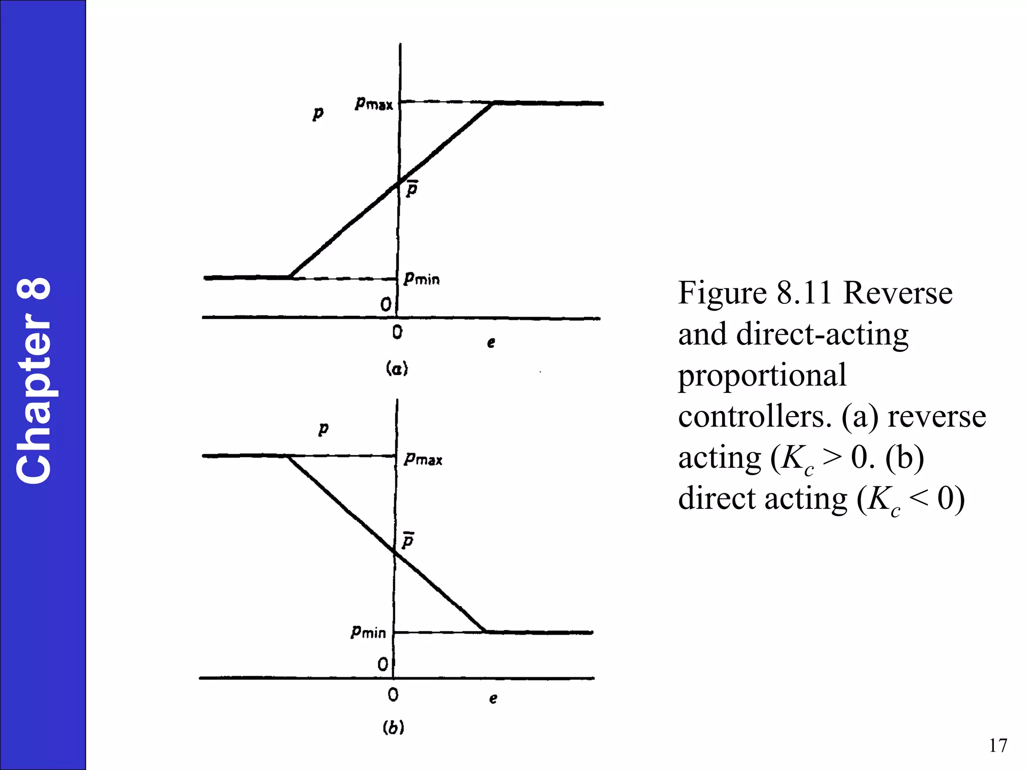
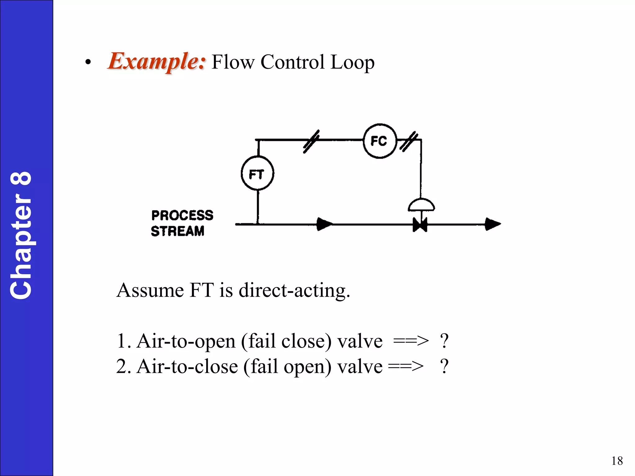
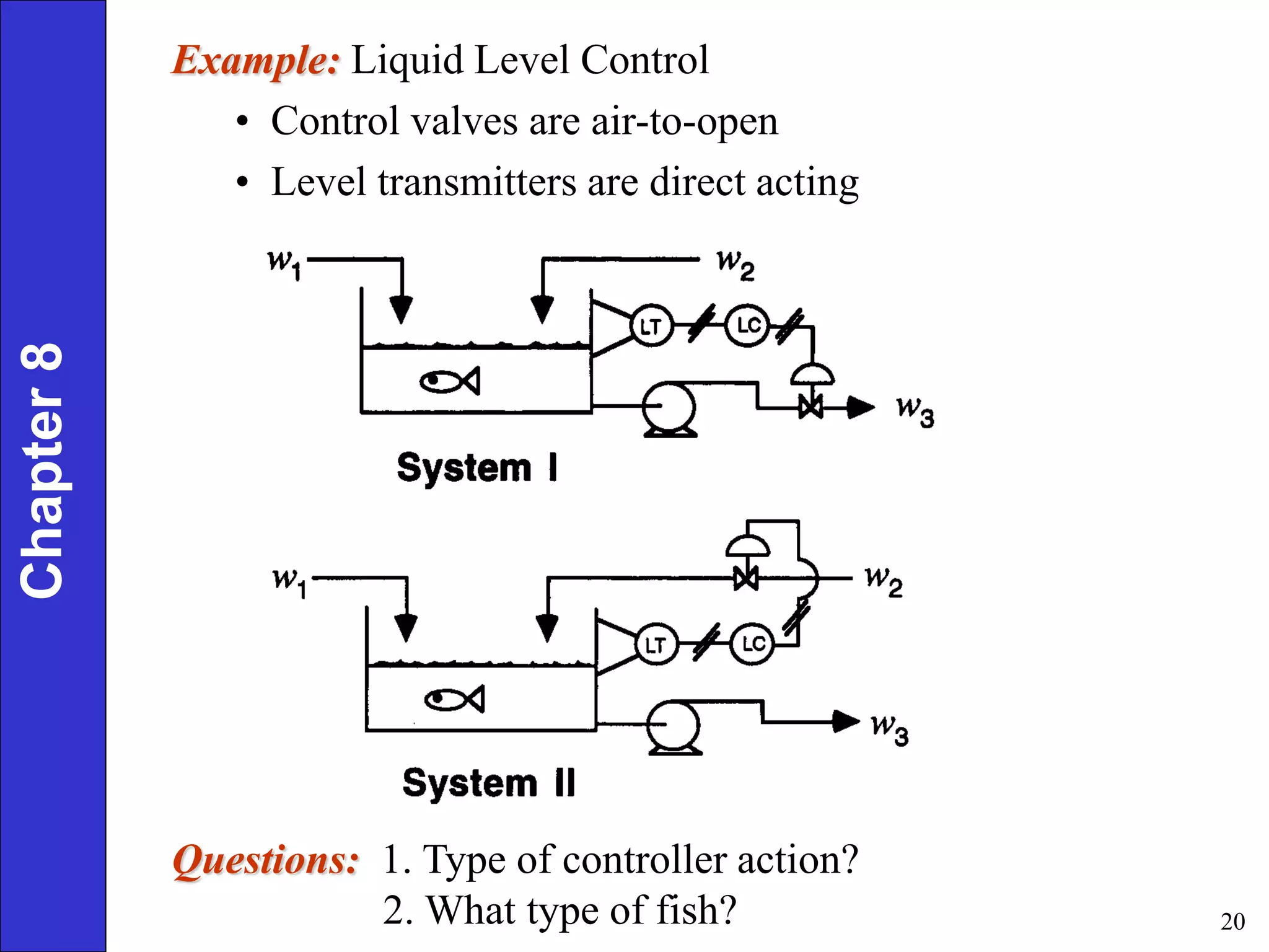
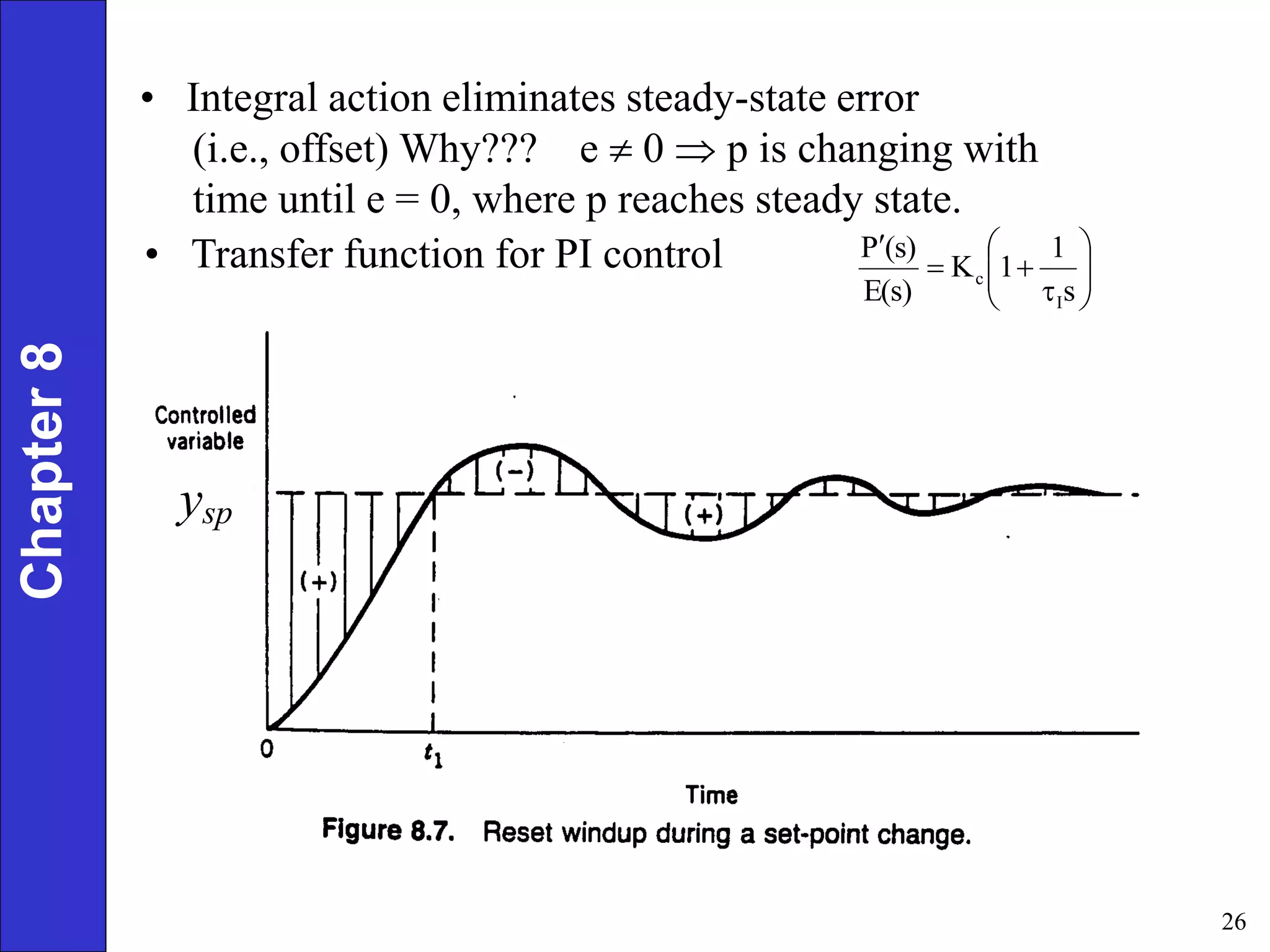
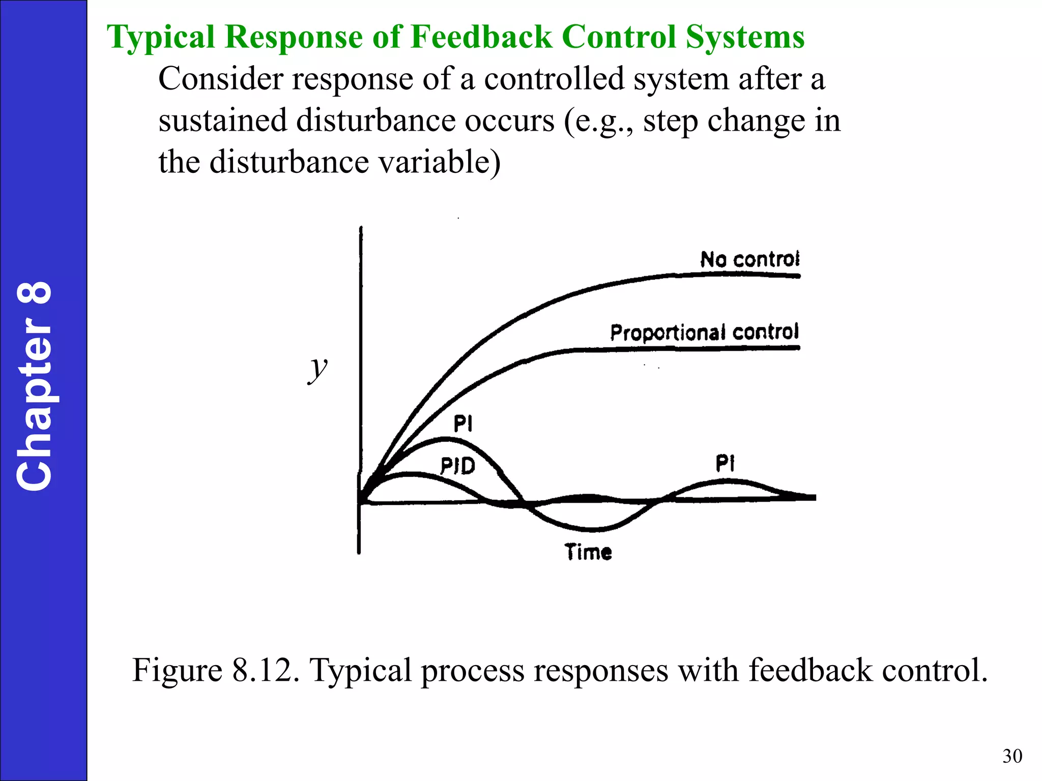
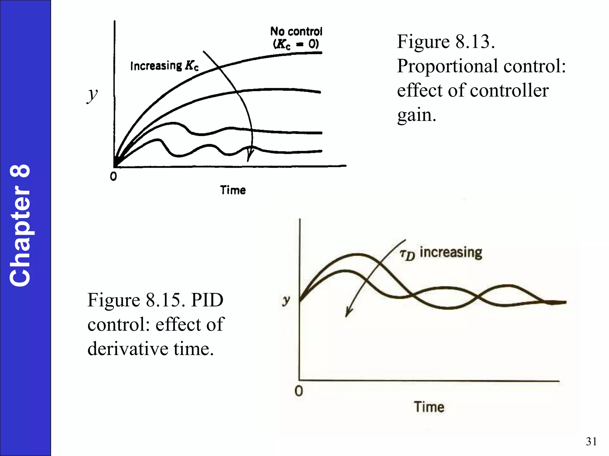
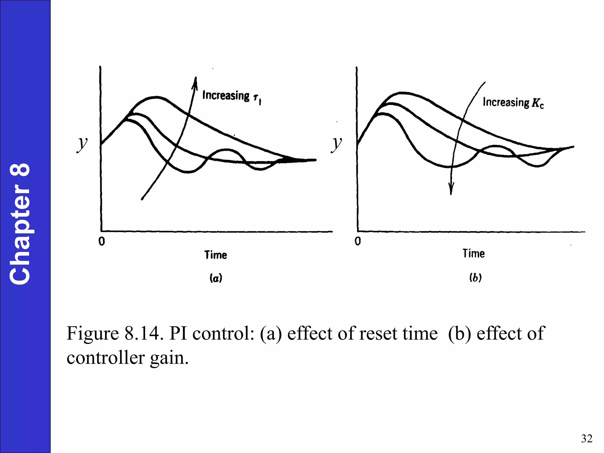
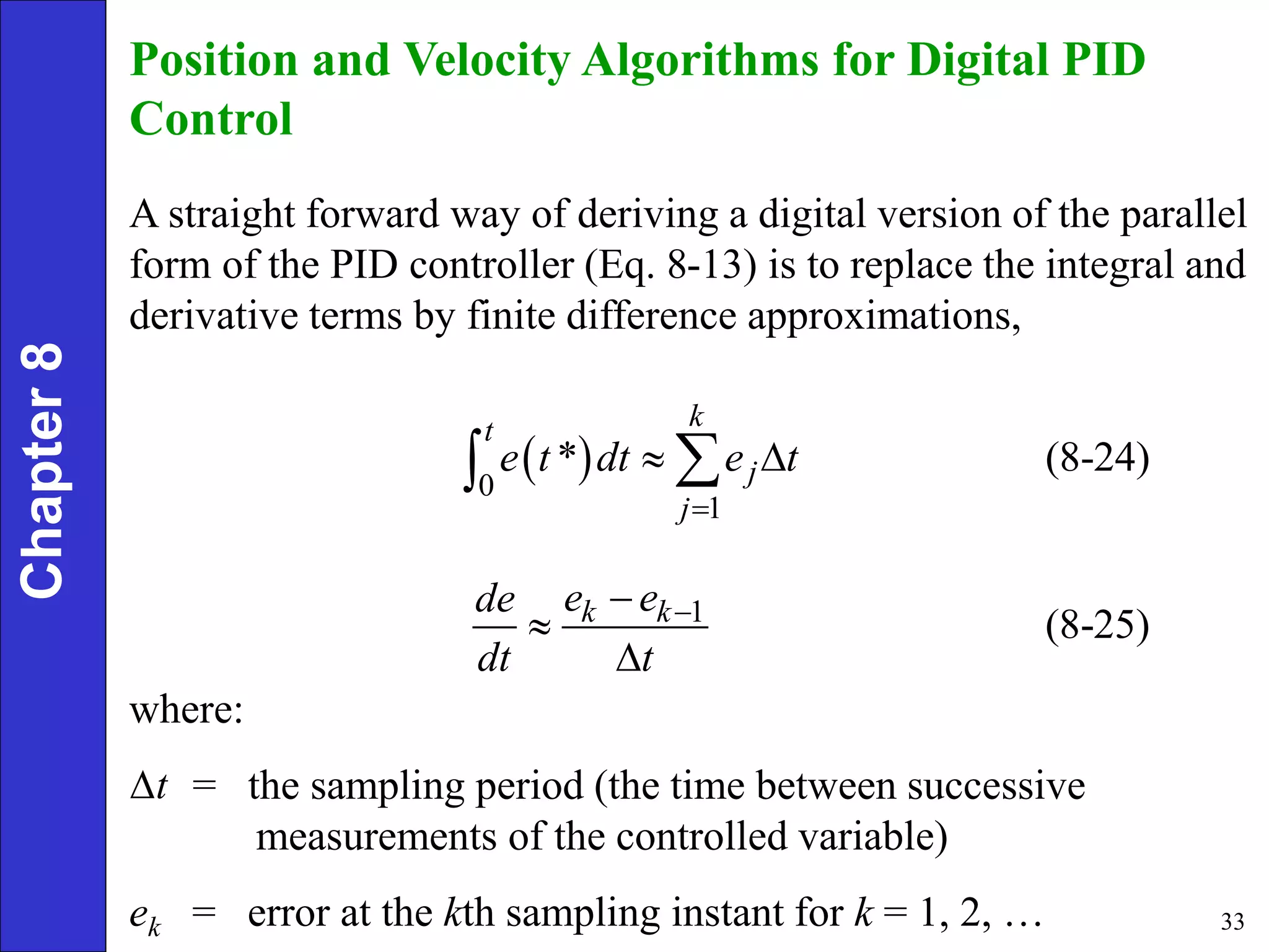
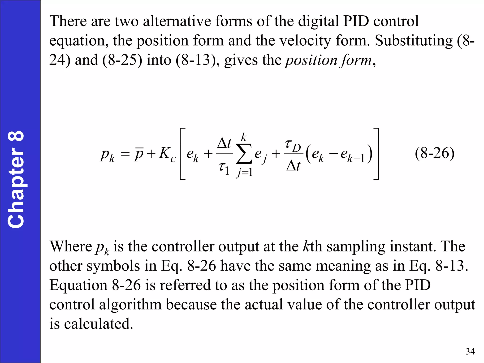
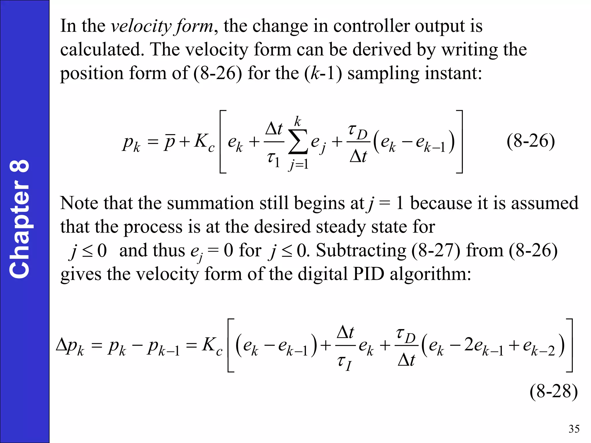
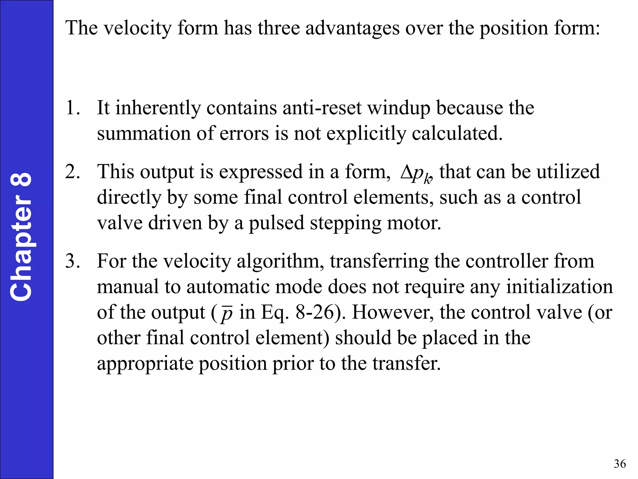
1. 1
Chapter
8
Figure 8.1 Schematic diagram for a stirred-tank blending
system.
Feedback Controllers

2. 2
Chapter
8 Basic Control Modes
Next we consider the three basic control modes starting with the
simplest mode, proportional control.
Proportional Control
In feedback control, the objective is to reduce the error signal to
zero where
      (8-1)
sp m
e t y t y t
 
and
 
 
 
error signal
set point
measured value of the controlled variable
(or equivalent signal from the sensor/transmitter)
sp
m
e t
y t
y t




3. 3
Chapter
8 Although Eq. 8-1 indicates that the set point can be time-varying,
in many process control problems it is kept constant for long
periods of time.
For proportional control, the controller output is proportional to
the error signal,
    (8-2)
c
p t p K e t
 
where:
  controller output
bias (steady-state) value
controller gain (usually dimensionless)
c
p t
p
K




4. 4
Chapter
8

5. 5
Chapter
8 The key concepts behind proportional control are the following:
1. The controller gain can be adjusted to make the controller
output changes as sensitive as desired to deviations between
set point and controlled variable;
2. the sign of Kc can be chosed to make the controller output
increase (or decrease) as the error signal increases.
For proportional controllers, bias can be adjusted, a procedure
referred to as manual reset.
Some controllers have a proportional band setting instead of a
controller gain. The proportional band PB (in %) is defined as
p
100%
(8-3)
c
PB
K

6. 6
Chapter
8 In order to derive the transfer function for an ideal proportional
controller (without saturation limits), define a deviation variable
as
 
p t

    (8-4)
p t p t p
 
Then Eq. 8-2 can be written as
    (8-5)
c
p t K e t
 
The transfer function for proportional-only control:
 
 
(8-6)
c
P s
K
E s


An inherent disadvantage of proportional-only control is that a
steady-state error occurs after a set-point change or a sustained
disturbance.

7. 7
Chapter
8 Integral Control
For integral control action, the controller output depends on the
integral of the error signal over time,
   
0
1
* * (8-7)
τ
t
I
p t p e t dt
  
where , an adjustable parameter referred to as the integral time
or reset time, has units of time.
τI
Integral control action is widely used because it provides an
important practical advantage, the elimination of offset.
Consequently, integral control action is normally used in
conjunction with proportional control as the proportional-integral
(PI) controller:
     
0
1
* * (8-8)
τ
t
c
I
p t p K e t e t dt
 
  
 
 


8. 8
Chapter
8 The corresponding transfer function for the PI controller in
Eq. 8-8 is given by
 
 
τ 1
1
1 (8-9)
τ τ
I
c c
I I
P s s
K K
E s s s
    

  
   
   
Some commercial controllers are calibrated in terms of
(repeats per minute) rather than (minutes, or minutes per
repeat).
1/ τI
τI
Reset Windup
• An inherent disadvantage of integral control action is a
phenomenon known as reset windup or integral windup.
• Recall that the integral mode causes the controller output to
change as long as e(t*) ≠ 0 in Eq. 8-8.

9. 9
Chapter
8 • When a sustained error occurs, the integral term becomes
quite large and the controller output eventually saturates.
• Further buildup of the integral term while the controller is
saturated is referred to as reset windup or integral windup.
Derivative Control
The function of derivative control action is to anticipate the future
behavior of the error signal by considering its rate of change.
• The anticipatory strategy used by the experienced operator can
be incorporated in automatic controllers by making the
controller output proportional to the rate of change of the error
signal or the controlled variable.

10. 10
Chapter
8 • Thus, for ideal derivative action,
 
 
τ (8-10)
D
de t
p t p
dt
 
where , the derivative time, has units of time.
For example, an ideal PD controller has the transfer function:
τD
 
 
 
1 τ (8-11)
c D
P s
K s
E s

 
• By providing anticipatory control action, the derivative mode
tends to stabilize the controlled process.
• Unfortunately, the ideal proportional-derivative control
algorithm in Eq. 8-10 is physically unrealizable because it
cannot be implemented exactly.

11. 11
Chapter
8 • For analog controllers, the transfer function in (8-11) can be
approximated by
 
 
τ
1 (8-12)
ατ 1
D
c
D
P s s
K
E s s
  
 
 

 
where the constant α typically has a value between 0.05 and
0.2, with 0.1 being a common choice.
• In Eq. 8-12 the derivative term includes a derivative mode
filter (also called a derivative filter) that reduces the sensitivity
of the control calculations to high-frequency noise in the
measurement.

12. 12
Chapter
8 Proportional-Integral-Derivative (PID) Control
Now we consider the combination of the proportional, integral,
and derivative control modes as a PID controller.
• Many variations of PID control are used in practice.
• Next, we consider the three most common forms.
Parallel Form of PID Control
The parallel form of the PID control algorithm (without a
derivative filter) is given by
     
 
0
1
* * τ (8-13)
τ
t
c D
I
de t
p t p K e t e t dt
dt
 
   
 
 


13. 13
Chapter
8 The corresponding transfer function is:
 
 
1
1 τ (8-14)
τ
c D
I
P s
K s
E s s
  
  
 
 
Series Form of PID Control
Historically, it was convenient to construct early analog
controllers (both electronic and pneumatic) so that a PI element
and a PD element operated in series.
Commercial versions of the series-form controller have a
derivative filter that is applied to either the derivative term, as in
Eq. 8-12, or to the PD term, as in Eq. 8-15:
 
 
τ 1 τ 1
(8-15)
τ ατ 1
I D
c
I D
P s s s
K
E s s s
   
 
   

  

14. 14
Chapter
8 Expanded Form of PID Control
In addition to the well-known series and parallel forms, the
expanded form of PID control in Eq. 8-16 is sometimes used:
     
 
0
* * (8-16)
t
c I D
de t
p t p K e t K e t dt K
dt
   

Features of PID Controllers
Elimination of Derivative and Proportional Kick
• One disadvantage of the previous PID controllers is that a
sudden change in set point (and hence the error, e) will cause the
derivative term momentarily to become very large and thus
provide a derivative kick to the final control element.

15. 15
Chapter
8 • This sudden change is undesirable and can be avoided by basing
the derivative action on the measurement, ym, rather than on the
error signal, e.
• We illustrate the elimination of derivative kick by considering
the parallel form of PID control in Eq. 8-13.
• Replacing de/dt by –dym/dt gives
     
 
0
1
* * τ (8-17)
τ
t m
c D
I
dy t
p t p K e t e t dt
dt
 
   
 
 

Reverse or Direct Action
• The controller gain can be made either negative or positive.

16. 16
Chapter
8 • For proportional control, when Kc > 0, the controller output p(t)
increases as its input signal ym(t) decreases, as can be seen by
combining Eqs. 8-2 and 8-1:
      (8-22)
c sp m
p t p K y t y t
 
  
 
• This controller is an example of a reverse-acting controller.
• When Kc < 0, the controller is said to be direct acting because
the controller output increases as the input increases.
• Equations 8-2 through 8-16 describe how controllers perform
during the automatic mode of operation.
• However, in certain situations the plant operator may decide to
override the automatic mode and adjust the controller output
manually.

17. 17
Chapter
8
Figure 8.11 Reverse
and direct-acting
proportional
controllers. (a) reverse
acting (Kc > 0. (b)
direct acting (Kc < 0)

18. 18
• Example: Flow Control Loop
Assume FT is direct-acting.
1. Air-to-open (fail close) valve ==> ?
2. Air-to-close (fail open) valve ==> ?
Chapter
8

19. 19
Automatic and Manual Control Modes
• Automatic Mode
Controller output, p(t), depends on e(t), controller
constants, and type of controller used.
( PI vs. PID etc.)
 Manual Mode
Controller output, p(t), is adjusted manually.
 Manual Mode is very useful when unusual
conditions exist:
plant start-up
plant shut-down
emergencies
• Percentage of controllers "on manual” ??
(30% in 2001, Honeywell survey)
Chapter
8

20. 20
Example: Liquid Level Control
• Control valves are air-to-open
• Level transmitters are direct acting
Chapter
8
Questions: 1. Type of controller action?
2. What type of fish?

21. 21
On-Off Controllers
• Simple
• Cheap
• Used In residential heating and domestic refrigerators
• Limited use in process control due to continuous
cycling of controlled variable  excessive wear
on control valve.
Chapter
8

22. 22
On-Off Controllers (continued)
Synonyms:
“two-position” or “bang-bang” controllers.
Controller output has two possible values.
Chapter
8

23. 23
Practical case (dead band)
Chapter
8

24. 24
Chapter
8

25. 25











 
t
0
I
c t
d
)
t
(
e
1
)
t
(
e
K
p
)
t
(
p
Proportional-Integral (PI) Control
• Response to unit step change in e:
Chapter
8
Figure 8.6. Response of proportional-integral controller to
unit step change in e(t).

26. 26
ysp
Chapter
8
• Integral action eliminates steady-state error
(i.e., offset) Why??? e  0  p is changing with
time until e = 0, where p reaches steady state.












s
1
1
K
E(s)
(s)
P
I
c
• Transfer function for PI control

27. 27
Derivative Control Action
 Ideal derivative action
 Used to improve dynamic response of the
controlled variable
 Derivative kick (use db/dt )
 Use alone?
 Some controllers are calibrated in 1/I
("repeats per minute") instead of I .
p
dt
de
p
)
t
(
p D



Chapter
8
 For PI controllers, is not adjustable.

28. 28
PID Controller
 Ideal controller













 
t
0
D
I
c
dt
de
t
d
)
t
(
e
1
)
t
(
e
K
p
)
t
(
p














s
s
1
1
K
E(s)
(s)
P
D
I
c
Chapter
8
• Transfer function (ideal)
 Transfer function (actual)
α = small number (0.05 to 0.20)

























1
s
1
s
s
1
s
K
E(s)
(s)
P
D
D
I
I
c
lead / lag units

29. 29
PID - Most complicated to tune (Kc, I, D) .
- Better performance than PI
- No offset
- Derivative action may be affected by noise
PI - More complicated to tune (Kc, I) .
- Better performance than P
- No offset
- Most popular FB controller
P - Simplest controller to tune (Kc).
- Offset with sustained disturbance or setpoint
change.
Controller Comparison
Chapter
8

30. 30
y
Typical Response of Feedback Control Systems
Consider response of a controlled system after a
sustained disturbance occurs (e.g., step change in
the disturbance variable)
Chapter
8
Figure 8.12. Typical process responses with feedback control.

31. 31
y
Chapter
8
Figure 8.13.
Proportional control:
effect of controller
gain.
Figure 8.15. PID
control: effect of
derivative time.

32. 32
y y
Chapter
8
Figure 8.14. PI control: (a) effect of reset time (b) effect of
controller gain.

33. 33
Chapter
8 Position and Velocity Algorithms for Digital PID
Control
A straight forward way of deriving a digital version of the parallel
form of the PID controller (Eq. 8-13) is to replace the integral and
derivative terms by finite difference approximations,
 
0
1
* (8-24)
k
t
j
j
e t dt e t

 


1
(8-25)
k k
e e
de
dt t




where:
= the sampling period (the time between successive
measurements of the controlled variable)
ek = error at the kth sampling instant for k = 1, 2, …
t


34. 34
Chapter
8 There are two alternative forms of the digital PID control
equation, the position form and the velocity form. Substituting (8-
24) and (8-25) into (8-13), gives the position form,
 
1
1 1
(8-26)
k
D
k c k j k k
j
t
p p K e e e e
t

 

 

    
 

 
 

Where pk is the controller output at the kth sampling instant. The
other symbols in Eq. 8-26 have the same meaning as in Eq. 8-13.
Equation 8-26 is referred to as the position form of the PID
control algorithm because the actual value of the controller output
is calculated.

35. 35
Chapter
8
 
1
1 1
(8-26)
k
D
k c k j k k
j
t
p p K e e e e
t

 

 

    
 

 
 

Note that the summation still begins at j = 1 because it is assumed
that the process is at the desired steady state for
and thus ej = 0 for . Subtracting (8-27) from (8-26)
gives the velocity form of the digital PID algorithm:
In the velocity form, the change in controller output is
calculated. The velocity form can be derived by writing the
position form of (8-26) for the (k-1) sampling instant:
0
j  0
j 
   
1 1 1 2
2
(8-28)
D
k k k c k k k k k k
I
t
p p p K e e e e e e
t


   
 

        
 

 

36. 36
Chapter
8 The velocity form has three advantages over the position form:
1. It inherently contains anti-reset windup because the
summation of errors is not explicitly calculated.
2. This output is expressed in a form, , that can be utilized
directly by some final control elements, such as a control
valve driven by a pulsed stepping motor.
3. For the velocity algorithm, transferring the controller from
manual to automatic mode does not require any initialization
of the output ( in Eq. 8-26). However, the control valve (or
other final control element) should be placed in the
appropriate position prior to the transfer.
k
p

p