Download as PDF, PPTX

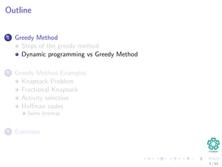


![You have two versions
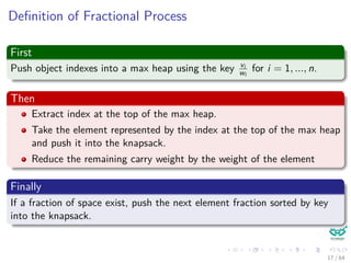
0-1 knapsack problem
You have to either take an item or not take it, you cannot take a
fraction of it.
Thus, elements in the vector are xi ∈ {0, 1} with i = 1, ..., n.
Fractional knapsack problem
Like the 0-1 knapsack problem, but you can take a fraction of an item.
Thus, elements in the vector are xi ∈ [0, 1] with i = 1, ..., n.
10 / 64](https://image.slidesharecdn.com/12greeddymethod-150324001342-conversion-gate01/85/12-Greeddy-Method-15-320.jpg)
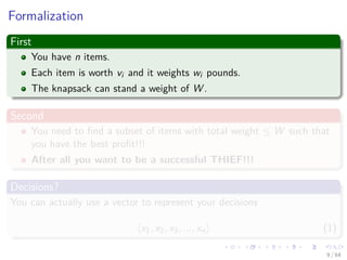
![You have two versions
0-1 knapsack problem
You have to either take an item or not take it, you cannot take a
fraction of it.
Thus, elements in the vector are xi ∈ {0, 1} with i = 1, ..., n.
Fractional knapsack problem
Like the 0-1 knapsack problem, but you can take a fraction of an item.
Thus, elements in the vector are xi ∈ [0, 1] with i = 1, ..., n.
10 / 64](https://image.slidesharecdn.com/12greeddymethod-150324001342-conversion-gate01/85/12-Greeddy-Method-16-320.jpg)


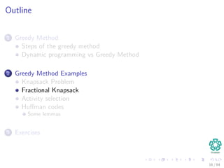

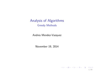
![Theorem about Greedy Choice
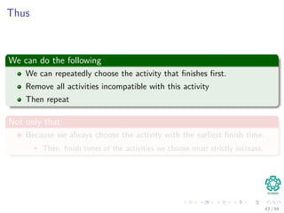
Theorem
The greedy choice, which always selects the object with better ratio
value/weight, always finds an optimal solution to the Fractional Knapsack
problem.
Proof
Constraints:
xi ∈ [0, 1]
18 / 64](https://image.slidesharecdn.com/12greeddymethod-150324001342-conversion-gate01/85/12-Greeddy-Method-30-320.jpg)
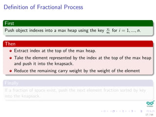
![Theorem about Greedy Choice
Theorem
The greedy choice, which always selects the object with better ratio
value/weight, always finds an optimal solution to the Fractional Knapsack
problem.
Proof
Constraints:
xi ∈ [0, 1]
18 / 64](https://image.slidesharecdn.com/12greeddymethod-150324001342-conversion-gate01/85/12-Greeddy-Method-31-320.jpg)
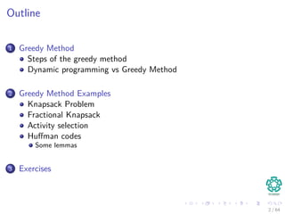
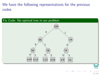
![Fractional Greedy
FRACTIONAL-KNAPSACK(W , w, v)
1 for i = 1 to n do x [i] = 0
2 weight = 0
3 // Use a Max-Heap
4 T = Build-Max-Heap(v/w)
5 while weight < W do
6 i = T.Heap-Extract-Max()
7 if (weight + w[i] ≤ W ) do
8 x [i] = 1
9 weight = weight + w[i]
10 else
11 x [i] = W −weight
w[i]
12 weight = W
13 return x
19 / 64](https://image.slidesharecdn.com/12greeddymethod-150324001342-conversion-gate01/85/12-Greeddy-Method-32-320.jpg)


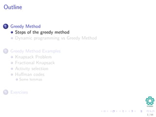
![Recursive Formulation
Recursive Formulation
c[i, j] =
0 if Sij = ∅
max
i<k<j
ak ∈Sij
c[i, k] + c[k, j] + 1 if Sij = ∅
Did you notice that you can use Dynamic Programming?
38 / 64](https://image.slidesharecdn.com/12greeddymethod-150324001342-conversion-gate01/85/12-Greeddy-Method-64-320.jpg)
![Recursive Formulation
Recursive Formulation
c[i, j] =
0 if Sij = ∅
max
i<k<j
ak ∈Sij
c[i, k] + c[k, j] + 1 if Sij = ∅
Did you notice that you can use Dynamic Programming?
38 / 64](https://image.slidesharecdn.com/12greeddymethod-150324001342-conversion-gate01/85/12-Greeddy-Method-65-320.jpg)


![Recursive Activity Selector
REC-ACTIVITY-SELECTOR(s, f , k, n) - Entry Point (s, f , 0, n)
1 m = k + 1
2 // find the first activity in Sk to finish
3 while m ≤ n and s [m] < f [k]
4 m = m + 1
5 if m ≤ n
6 return {am} ∪REC-ACTIVITY-SELECTOR(s, f , m, n)
7 else return ∅
46 / 64](https://image.slidesharecdn.com/12greeddymethod-150324001342-conversion-gate01/85/12-Greeddy-Method-79-320.jpg)

![We can do more...
GREEDY-ACTIVITY-SELECTOR(s, f , n)
1 n = s.length
2 A={a1}
3 k = 1
4 for m = 2 to n
5 if s [m] ≥ f [k]
6 A=A∪ {am}
7 k = m
8 return A
Complexity of the algorithm
Θ(n)
Note: Clearly, we are not taking into account the sorting of the
activities.
48 / 64](https://image.slidesharecdn.com/12greeddymethod-150324001342-conversion-gate01/85/12-Greeddy-Method-81-320.jpg)
![We can do more...
GREEDY-ACTIVITY-SELECTOR(s, f , n)
1 n = s.length
2 A={a1}
3 k = 1
4 for m = 2 to n
5 if s [m] ≥ f [k]
6 A=A∪ {am}
7 k = m
8 return A
Complexity of the algorithm
Θ(n)
Note: Clearly, we are not taking into account the sorting of the
activities.
48 / 64](https://image.slidesharecdn.com/12greeddymethod-150324001342-conversion-gate01/85/12-Greeddy-Method-82-320.jpg)


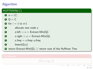
![Cost in the number of bits to represent the text
Fix Code
3 × 100, 000 = 300, 000 bits (2)
Variable Code
[45 × 1 + 13 × 3 + 12 × 3 + 16 × 3 + ...
9 × 4 + 5 × 4] × 1000 = 224, 000 bits
54 / 64](https://image.slidesharecdn.com/12greeddymethod-150324001342-conversion-gate01/85/12-Greeddy-Method-91-320.jpg)
![Cost in the number of bits to represent the text
Fix Code
3 × 100, 000 = 300, 000 bits (2)
Variable Code
[45 × 1 + 13 × 3 + 12 × 3 + 16 × 3 + ...
9 × 4 + 5 × 4] × 1000 = 224, 000 bits
54 / 64](https://image.slidesharecdn.com/12greeddymethod-150324001342-conversion-gate01/85/12-Greeddy-Method-92-320.jpg)


This document discusses greedy algorithms and provides examples of their application. It begins with an outline and overview of the greedy method approach. Key steps are presented, including determining optimal substructure, developing recursive and iterative solutions, and proving greedy choices are optimal. Examples analyzed include knapsack problems, activity selection, and Huffman codes. Details are given on solving fractional knapsack problems greedily. The optimal substructure of activity selection problems is explored.