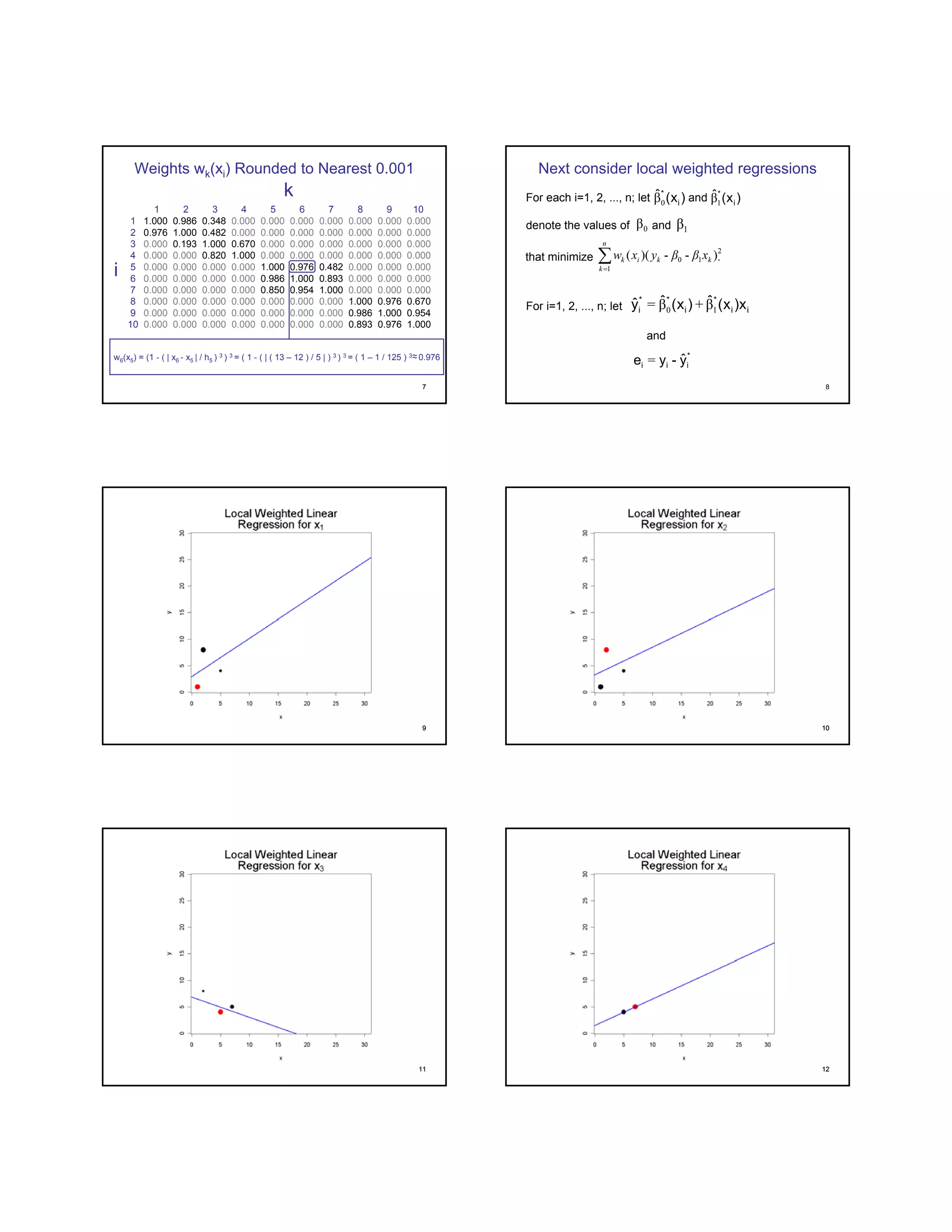
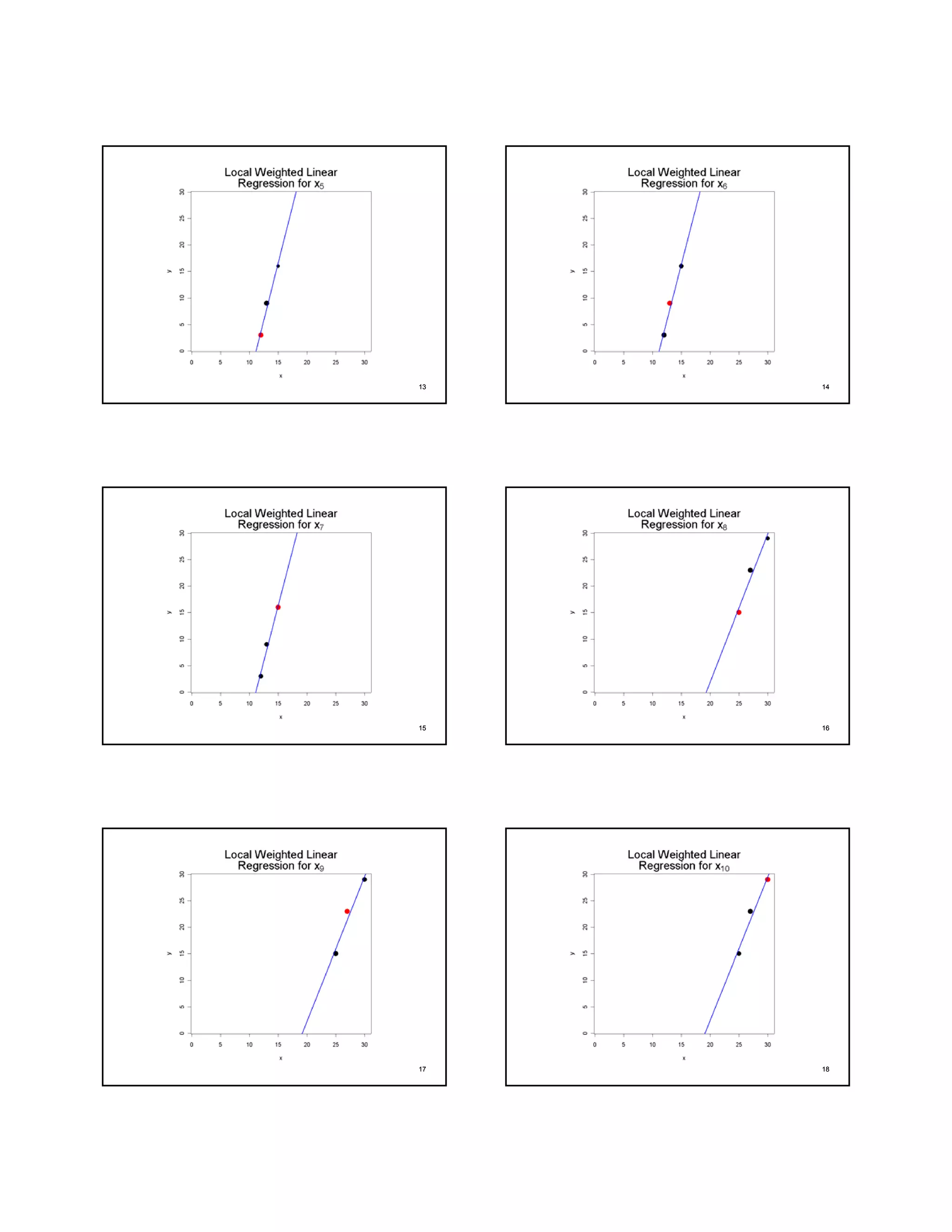
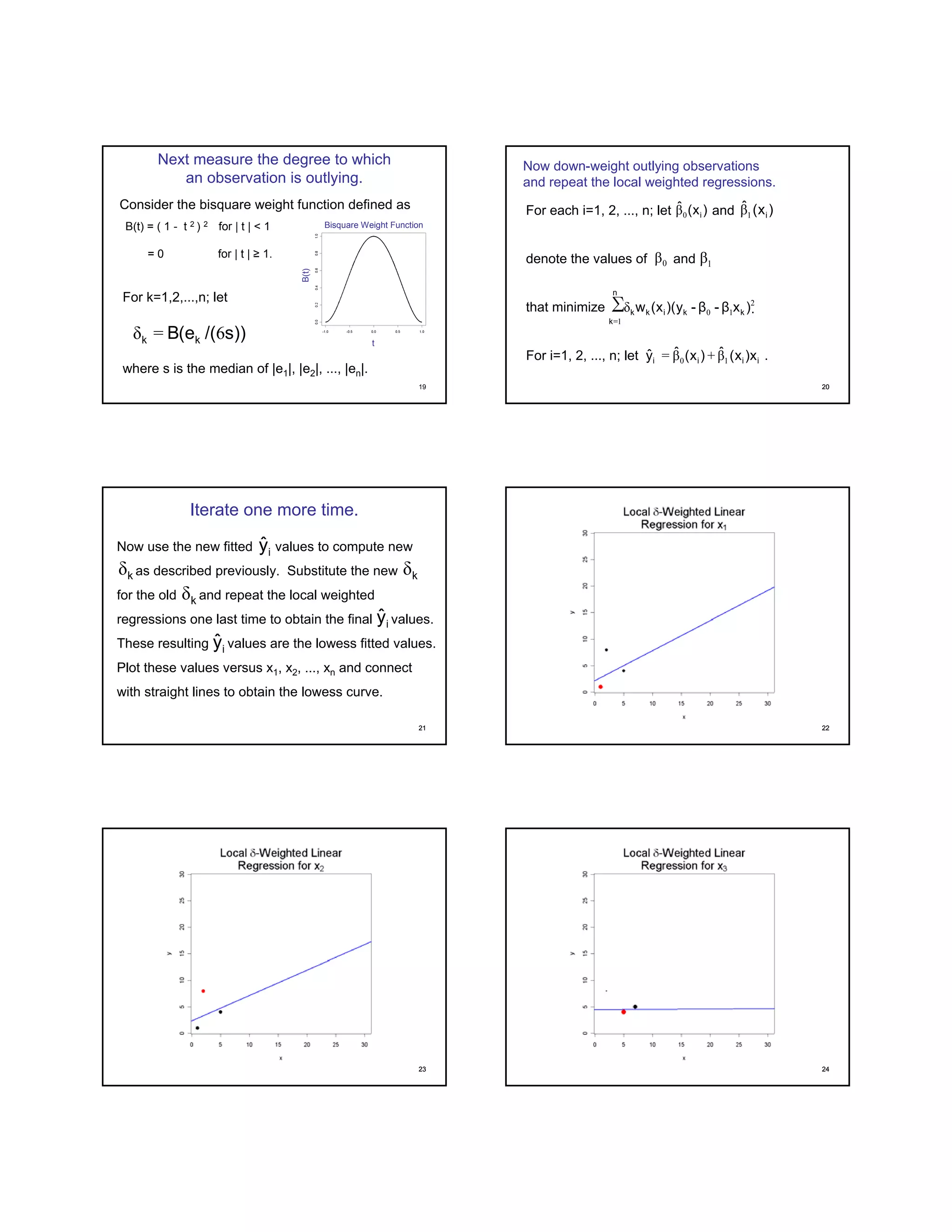
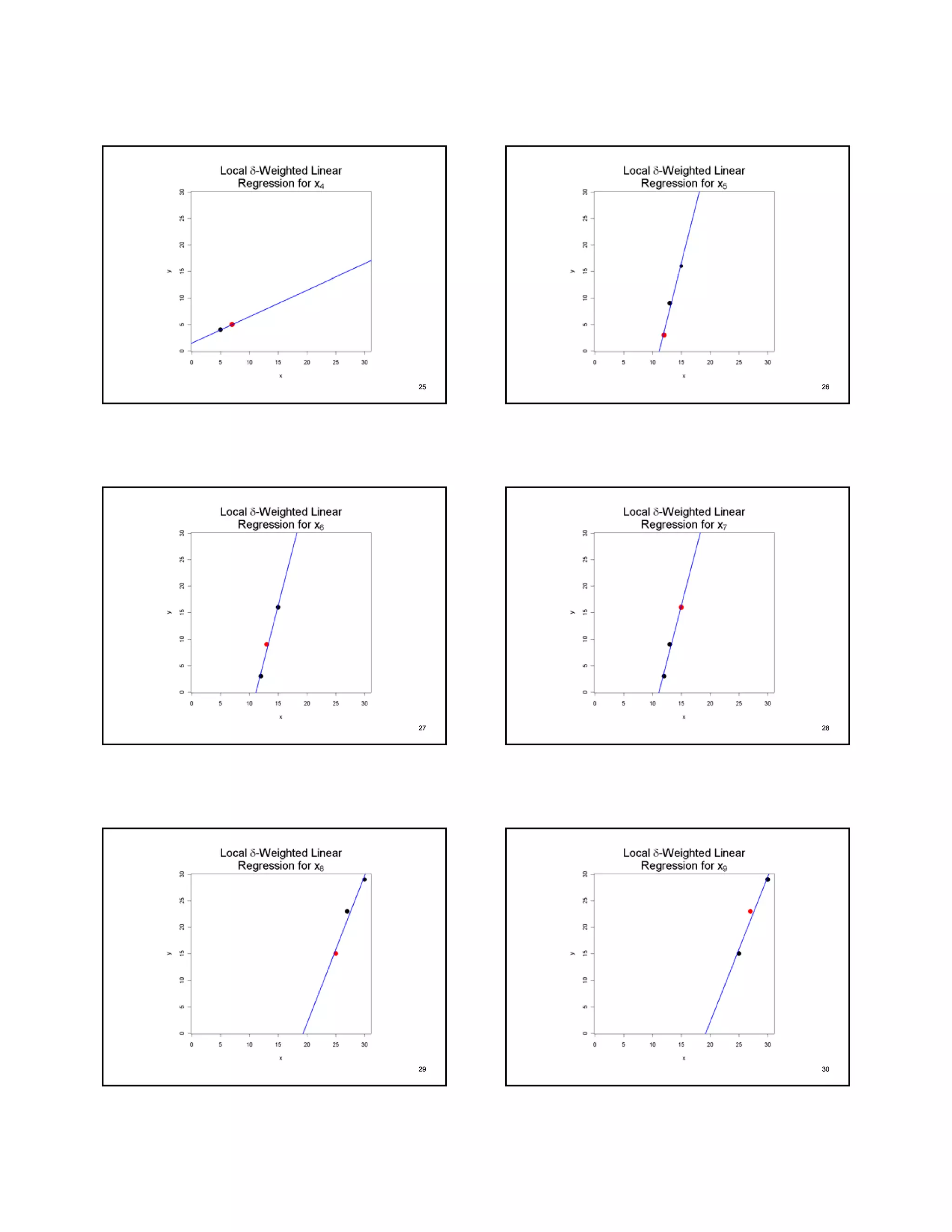
11
The LOWESS Smoother
1/19/2011
Copyright © 2011 Dan Nettleton
22
LOWESS
“lowess” stands for
LOcally WEighted polynomial regreSSion.
The original reference for lowess is
Cleveland, W. S. (1979). Robust locally weighted
regression and smoothing scatterplots.
JASA 74 829-836.
33
How is the lowess curve determined?
Consider the tricube weight function defined as
Suppose we have data points (x1,y1), (x2,y2),...(xn,yn).
Let 0 < f ≤ 1 denote a fraction that will determine the smoothness of the curve.
Let r = n*f rounded to the nearest integer.
t
T(t)
Tricube Weight Function
For i=1, ..., n; let hi be the rth smallest
number among |xi-x1|, |xi-x2|, ..., |xi-xn|.
T(t) = ( 1 - | t | 3 ) 3 for | t | < 1
= 0 for | t | ≥ 1.
For k=1, 2, ..., n; let wk(xi)=T( ( xk – xi ) / hi ).
44
An Example
i 1 2 3 4 5 6 7 8 9 10
xi 1 2 5 7 12 13 15 25 27 30
yi 1 8 4 5 3 9 16 15 23 29
x
y
Suppose a
lowess curve
will be fit
to this data
with f=0.4.
55
Table Containing |xi-xj| Values
x1 x2 x3 x4 x5 x6 x7 x8 x9 x10
x1 0 1 4 6 11 12 14 24 26 29
x2 1 0 3 5 10 11 13 23 25 28
x3 4 3 0 2 7 8 10 20 22 25
x4 6 5 2 0 5 6 8 18 20 23
x5 11 10 7 5 0 1 3 13 15 18
x6 12 11 8 6 1 0 2 12 14 17
x7 14 13 10 8 3 2 0 10 12 15
x8 24 23 20 18 13 12 10 0 2 5
x9 26 25 22 20 15 14 12 2 0 3
x10 29 28 25 23 18 17 15 5 3 0
66
Calculation of hi from |xi-xj| Values
x1 x2 x3 x4 x5 x6 x7 x8 x9 x10
x1 0 1 4 6 11 12 14 24 26 29 h1= 6
x2 1 0 3 5 10 11 13 23 25 28 h2= 5
x3 4 3 0 2 7 8 10 20 22 25 h3= 4
x4 6 5 2 0 5 6 8 18 20 23 h4= 5
x5 11 10 7 5 0 1 3 13 15 18 h5= 5
x6 12 11 8 6 1 0 2 12 14 17 h6= 6
x7 14 13 10 8 3 2 0 10 12 15 h7= 8
x8 24 23 20 18 13 12 10 0 2 5 h8=10
x9 26 25 22 20 15 14 12 2 0 3 h9=12
x10 29 28 25 23 18 17 15 5 3 0 h10=15
n=10, f=0.4 r=4
77
Weights wk(xi) Rounded to Nearest 0.001
1 2 3 4 5 6 7 8 9 10
1 1.000 0.986 0.348 0.000 0.000 0.000 0.000 0.000 0.000 0.000
2 0.976 1.000 0.482 0.000 0.000 0.000 0.000 0.000 0.000 0.000
3 0.000 0.193 1.000 0.670 0.000 0.000 0.000 0.000 0.000 0.000
4 0.000 0.000 0.820 1.000 0.000 0.000 0.000 0.000 0.000 0.000
5 0.000 0.000 0.000 0.000 1.000 0.976 0.482 0.000 0.000 0.000
6 0.000 0.000 0.000 0.000 0.986 1.000 0.893 0.000 0.000 0.000
7 0.000 0.000 0.000 0.000 0.850 0.954 1.000 0.000 0.000 0.000
8 0.000 0.000 0.000 0.000 0.000 0.000 0.000 1.000 0.976 0.670
9 0.000 0.000 0.000 0.000 0.000 0.000 0.000 0.986 1.000 0.954
10 0.000 0.000 0.000 0.000 0.000 0.000 0.000 0.893 0.976 1.000
i
k
w6(x5) = (1 - ( | x6 - x5 | / h5 ) 3 ) 3 = ( 1 - ( | ( 13 – 12 ) / 5 | ) 3 ) 3 = ( 1 – 1 / 125 ) 3 0.976~~
8
Next consider local weighted regressions
)x(ˆ i
*
0β
∑=
n
k
kkik xββyxw
1
2
10 )--)((
For each i=1, 2, ..., n; let and
denote the values of and0β 1β
that minimize .
ii
*
i
**
i x)x(ˆ)x(ˆyˆ 10 β+β=For i=1, 2, ..., n; let
*
iii yˆ-ye =
)x(ˆ i
*
1β
and
99 1010
1111 1212
1313 1414
1515 1616
1717 1818
19
19
Next measure the degree to which
an observation is outlying.
))s/(e(B kk 6=δ
Consider the bisquare weight function defined as
B(t) = ( 1 - t 2 ) 2 for | t | < 1
= 0 for | t | ≥ 1.
B(t)
Bisquare Weight Function
t
For k=1,2,...,n; let
where s is the median of |e1|, |e2|, ..., |en|.
2020
)x(ˆ i1β
∑
1
2
10
n
k
kkikk )xβ-β-y)(x(w
=
δ
)x(ˆ i0βFor each i=1, 2, ..., n; let and
denote the values of and
that minimize
0β 1β
iiii x)x(ˆ)x(ˆyˆ 10 β+β=For i=1, 2, ..., n; let
.
.
Now down-weight outlying observations
and repeat the local weighted regressions.
2121
Iterate one more time.
Now use the new fitted values to compute new
as described previously. Substitute the new
for the old and repeat the local weighted
regressions one last time to obtain the final values.
These resulting values are the lowess fitted values.
Plot these values versus x1, x2, ..., xn and connect
with straight lines to obtain the lowess curve.
iyˆ
kδ kδ
kδ
iyˆ
iyˆ
2222
2323 2424
2525 2626
2727 2828
2929 3030
3131 3232
Plot Showing All 10 Lines and Predicted Values
after One More Iteration
3333
The Lowess Curve
3434
lowess in R
o=lowess(x,y,f=0.4)
plot(x,y)
lines(o$x,o$y,col=2,lwd=2)
o$x will be a vector containing the x values.
o$y will contain the lowess fitted values for the values in o$x.
f controls the fraction of the data used to obtain each fitted value.
35
o=lowess(y~x,f=.2)
plot(fossil)
lines(o,lwd=2)
#See also the function 'loess' which has more
#capabilities than 'lowess'.
36

08lowess

  • 1.
    11 The LOWESS Smoother 1/19/2011 Copyright© 2011 Dan Nettleton 22 LOWESS “lowess” stands for LOcally WEighted polynomial regreSSion. The original reference for lowess is Cleveland, W. S. (1979). Robust locally weighted regression and smoothing scatterplots. JASA 74 829-836. 33 How is the lowess curve determined? Consider the tricube weight function defined as Suppose we have data points (x1,y1), (x2,y2),...(xn,yn). Let 0 < f ≤ 1 denote a fraction that will determine the smoothness of the curve. Let r = n*f rounded to the nearest integer. t T(t) Tricube Weight Function For i=1, ..., n; let hi be the rth smallest number among |xi-x1|, |xi-x2|, ..., |xi-xn|. T(t) = ( 1 - | t | 3 ) 3 for | t | < 1 = 0 for | t | ≥ 1. For k=1, 2, ..., n; let wk(xi)=T( ( xk – xi ) / hi ). 44 An Example i 1 2 3 4 5 6 7 8 9 10 xi 1 2 5 7 12 13 15 25 27 30 yi 1 8 4 5 3 9 16 15 23 29 x y Suppose a lowess curve will be fit to this data with f=0.4. 55 Table Containing |xi-xj| Values x1 x2 x3 x4 x5 x6 x7 x8 x9 x10 x1 0 1 4 6 11 12 14 24 26 29 x2 1 0 3 5 10 11 13 23 25 28 x3 4 3 0 2 7 8 10 20 22 25 x4 6 5 2 0 5 6 8 18 20 23 x5 11 10 7 5 0 1 3 13 15 18 x6 12 11 8 6 1 0 2 12 14 17 x7 14 13 10 8 3 2 0 10 12 15 x8 24 23 20 18 13 12 10 0 2 5 x9 26 25 22 20 15 14 12 2 0 3 x10 29 28 25 23 18 17 15 5 3 0 66 Calculation of hi from |xi-xj| Values x1 x2 x3 x4 x5 x6 x7 x8 x9 x10 x1 0 1 4 6 11 12 14 24 26 29 h1= 6 x2 1 0 3 5 10 11 13 23 25 28 h2= 5 x3 4 3 0 2 7 8 10 20 22 25 h3= 4 x4 6 5 2 0 5 6 8 18 20 23 h4= 5 x5 11 10 7 5 0 1 3 13 15 18 h5= 5 x6 12 11 8 6 1 0 2 12 14 17 h6= 6 x7 14 13 10 8 3 2 0 10 12 15 h7= 8 x8 24 23 20 18 13 12 10 0 2 5 h8=10 x9 26 25 22 20 15 14 12 2 0 3 h9=12 x10 29 28 25 23 18 17 15 5 3 0 h10=15 n=10, f=0.4 r=4
  • 2.
    77 Weights wk(xi) Roundedto Nearest 0.001 1 2 3 4 5 6 7 8 9 10 1 1.000 0.986 0.348 0.000 0.000 0.000 0.000 0.000 0.000 0.000 2 0.976 1.000 0.482 0.000 0.000 0.000 0.000 0.000 0.000 0.000 3 0.000 0.193 1.000 0.670 0.000 0.000 0.000 0.000 0.000 0.000 4 0.000 0.000 0.820 1.000 0.000 0.000 0.000 0.000 0.000 0.000 5 0.000 0.000 0.000 0.000 1.000 0.976 0.482 0.000 0.000 0.000 6 0.000 0.000 0.000 0.000 0.986 1.000 0.893 0.000 0.000 0.000 7 0.000 0.000 0.000 0.000 0.850 0.954 1.000 0.000 0.000 0.000 8 0.000 0.000 0.000 0.000 0.000 0.000 0.000 1.000 0.976 0.670 9 0.000 0.000 0.000 0.000 0.000 0.000 0.000 0.986 1.000 0.954 10 0.000 0.000 0.000 0.000 0.000 0.000 0.000 0.893 0.976 1.000 i k w6(x5) = (1 - ( | x6 - x5 | / h5 ) 3 ) 3 = ( 1 - ( | ( 13 – 12 ) / 5 | ) 3 ) 3 = ( 1 – 1 / 125 ) 3 0.976~~ 8 Next consider local weighted regressions )x(ˆ i * 0β ∑= n k kkik xββyxw 1 2 10 )--)(( For each i=1, 2, ..., n; let and denote the values of and0β 1β that minimize . ii * i ** i x)x(ˆ)x(ˆyˆ 10 β+β=For i=1, 2, ..., n; let * iii yˆ-ye = )x(ˆ i * 1β and 99 1010 1111 1212
  • 3.
  • 4.
    19 19 Next measure thedegree to which an observation is outlying. ))s/(e(B kk 6=δ Consider the bisquare weight function defined as B(t) = ( 1 - t 2 ) 2 for | t | < 1 = 0 for | t | ≥ 1. B(t) Bisquare Weight Function t For k=1,2,...,n; let where s is the median of |e1|, |e2|, ..., |en|. 2020 )x(ˆ i1β ∑ 1 2 10 n k kkikk )xβ-β-y)(x(w = δ )x(ˆ i0βFor each i=1, 2, ..., n; let and denote the values of and that minimize 0β 1β iiii x)x(ˆ)x(ˆyˆ 10 β+β=For i=1, 2, ..., n; let . . Now down-weight outlying observations and repeat the local weighted regressions. 2121 Iterate one more time. Now use the new fitted values to compute new as described previously. Substitute the new for the old and repeat the local weighted regressions one last time to obtain the final values. These resulting values are the lowess fitted values. Plot these values versus x1, x2, ..., xn and connect with straight lines to obtain the lowess curve. iyˆ kδ kδ kδ iyˆ iyˆ 2222 2323 2424
  • 5.
  • 6.
    3131 3232 Plot ShowingAll 10 Lines and Predicted Values after One More Iteration 3333 The Lowess Curve 3434 lowess in R o=lowess(x,y,f=0.4) plot(x,y) lines(o$x,o$y,col=2,lwd=2) o$x will be a vector containing the x values. o$y will contain the lowess fitted values for the values in o$x. f controls the fraction of the data used to obtain each fitted value. 35 o=lowess(y~x,f=.2) plot(fossil) lines(o,lwd=2) #See also the function 'loess' which has more #capabilities than 'lowess'. 36