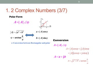
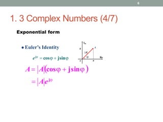
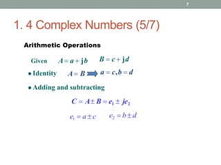
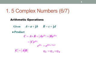
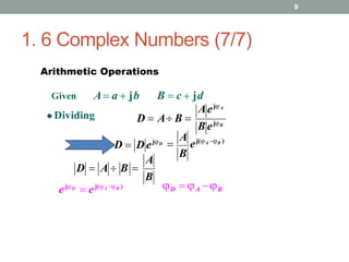
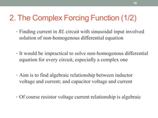
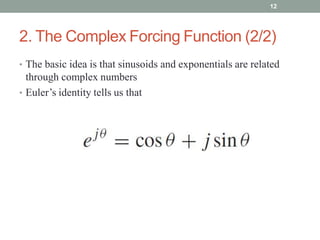
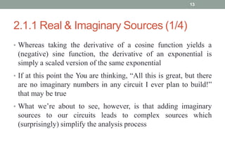
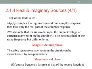
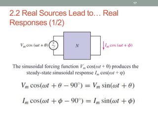
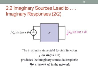
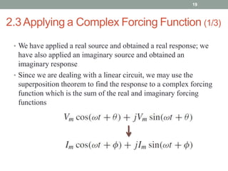
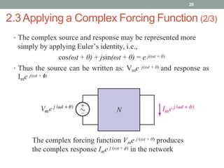
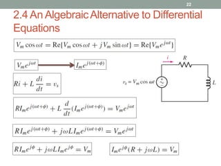
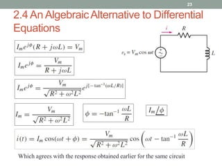
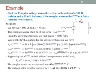
The document discusses complex numbers and their application to sinusoidal steady-state analysis of circuits. It introduces complex numbers in rectangular, polar, and exponential forms. It then explains how real sources produce real responses while imaginary sources produce imaginary responses. Applying a complex forcing function allows obtaining the full complex response, from which the real response can be extracted. This provides an algebraic alternative to solving differential equations. An example problem demonstrates finding the complex voltage across series R and L elements using this approach.

1. LECTURE 03
Chapter 10: Sinusoidal Steady-State Analysis
1

2. Lecture 03: Agenda
1. Complex Numbers
1. Types
2. Arithmetic Operations
2. The Complex Forcing Function
1. Real & Imaginary Sources
2. Real Sources Lead to… Real Responses
3. Imaginary Sources Lead to… Imaginary Responses
4. Applying a Complex Forcing Function
5. AnAlgebraicAlternative to Differential Equations
2

3. 1. Complex Numbers (1/7)
3
Rectangularform
Polar form
Exponential form
A a  jb
A| A|
A| A| ej
Three forms
•Arithmetic operations of complex numbers

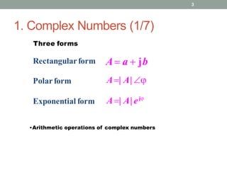
4. 1.1 Complex Numbers (2/7)
4
Rectangular form
A a  jb
j   1
a  Re[A]
b  Im[ A]
a
b
Im
Re
0
|A|

A
 Imaginary unit
 Real part
 Imaginary part
 Magnitude
 Angle
 Conjugate
a2
 b2
 A
2
 A  a2
 b2
a
  arctan
b
A  a  jb A  A AA  A2

5. 1. 2 Complex Numbers (3/7)
5
a
Re
0
|A|

Im
b
A
A  a2
 b2
a
  arctan
b
A| A|
a | A|cos
b | A|sin
 Conversion between Rectangular and polar
Polar Form
Conversion
A| A|
A  A cos  j A sin
 A cos  jsin
A a  jb
A  a2
b2
arctan
b
a

6. 1. 3 Complex Numbers (4/7)
6
A Acos  jsin
 Aej
 Euler’s Identity
ej
 cos  jsin a
b
Re
0
|A|

Im
A
Exponential form

7. 1. 4 Complex Numbers (5/7)
7
Arithmetic Operations
A a  jb
A B
Given
 Identity
B  c  jd
a  c,b  d
 Adding and subtracting
C  A B  e1  je2
e1  a  c e2  b  d

8. 1. 5 Complex Numbers (6/7)
8
Arithmetic Operations
A a  jb B  c  jd
Given
 Product
C  AB  AejA
 BejB
 C ejC
C  A B
ejC
 ej(AB )
C  A B

9. 1. 6 Complex Numbers (7/7)
9
B ejB
AejA
D  A B 
B
A
D  A  B 
ejD
 ej(AB ) D  A B
D  D ejD
B

A
ej(A B )
Arithmetic Operations
A a  jb B  c  jd
Given
 Dividing

10. 2. The Complex Forcing Function (1/2)
• Finding current in RL circuit with sinusoidal input involved
solution of non-homogenous differential equation
• It would be impractical to solve non-homogenous differential
equation for every circuit, especially a complex one
• Aim is to find algebraic relationship between inductor
voltage and current; and capacitor voltage and current
• Of course resistor voltage current relationship is algebraic
10

11. 2. The Complex Forcing Function (1/2)
• We introduce complex forcing function to emulate a
sinusoidal forcing function that will result into linear
algebraic equation instead of differential equation
• For linear circuits Steady State Response will follow the
shape of Forcing Function, therefore:
• DC source will produce constant response
• Sinusoidal source will result into Sinusoidal Response
• Exponential and Ramp input will produce exponential and
Ramp response respectively, in Steady State
11

12. 2. The Complex Forcing Function (2/2)
• The basic idea is that sinusoids and exponentials are related
through complex numbers
• Euler’s identity tells us that
12

13. 2.1.1 Real & Imaginary Sources (1/4)
• Whereas taking the derivative of a cosine function yields a
(negative) sine function, the derivative of an exponential is
simply a scaled version of the same exponential
• If at this point the You are thinking, “All this is great, but there
are no imaginary numbers in any circuit I ever plan to build!”
that may be true
• What we’re about to see, however, is that adding imaginary
sources to our circuits leads to complex sources which
(surprisingly) simplify the analysis process
13

14. 2.1.2 Real & Imaginary Sources (2/4)
• It might seem like a strange idea at first, but a moment’s
reflection should remind us that superposition requires any
imaginary sources we might add to cause only imaginary
responses, and real sources can only lead to real responses
• Thus, at any point, we should be able to separate the two by
simply taking the real part of any complex voltage or current
14

15. 2.1.3 Real & Imaginary Sources (3/4)
15
• Areal sinusoid will produce a real sinusoidal response
•An imaginary forcing function will produce imaginary
response
• Acomplex forcing function will produce complex response
• Real part corresponds to real response
• Imaginary part corresponds to imaginary response

16. 2.1.4 Real & Imaginary Sources (4/4)
16
Trick of the trade is to:
•Apply complex forcing function and find complex response
then take only the real part of the complex response
•We also note that for sinusoidal input the output (voltage or
current) at any point on the circuit will also be sinusoidal of the
same frequency but differ only in:
Magnitude and phase
Therefore response at any point on the circuit can be
characterized by two parameters:
Magnitude and phase
(Of course frequency is same as that of the source function)

17. 2.2 Real Sources Lead to… Real
Responses (1/2)
17
The sinusoidal forcing function Vm cos(ωt + θ) produces the
steady-state sinusoidal response Im cos(ωt + φ)

18. 2.2 Imaginary Sources Lead to . . .
Imaginary Responses (2/2)
18
The imaginary sinusoidal forcing function
jVm sin(ωt + θ)
produces the imaginary sinusoidal response
jIm sin(ωt + φ) in the network

19. 2.3Applying a Complex Forcing Function (1/3)
• We have applied a real source and obtained a real response; we
have also applied an imaginary source and obtained an
imaginary response
• Since we are dealing with a linear circuit, we may use the
superposition theorem to find the response to a complex forcing
function which is the sum of the real and imaginary forcing
functions
19

20. • The complex source and response may be represented more
simply by applying Euler’s identity, i.e.,
cos(ωt + θ) + jsin(ωt + θ) = e j(ωt + θ)
• Thus the source can be written as: Vme j(ωt + θ) and response as
Ime j(ωt + ϕ)
20
The complex forcing function Vme j (ωt + θ) produces
the complex response Ime j (ωt + ϕ) in the network
2.3Applying a Complex Forcing Function (2/3)

21. 2.3Applying a Complex Forcing Function (3/3)
• Again, linearity assures us that the real part of the complex
response is produced by the real part of the complex forcing
function, while the imaginary part of the response is caused by
the imaginary part of the complex forcing function
• Our plan is that instead of applying a real forcing function to
obtain the desired real response, we will substitute a complex
forcing function whose real part is the given real forcing
function; we expect to obtain a complex response whose real
part is the desired real response
• The advantage of this procedure is that the integrodifferential
equations describing the steady-state response of a circuit will
now become simple algebraic equations
21

22. 2.4An AlgebraicAlternative to Differential
Equations
22

23. 2.4An AlgebraicAlternative to Differential
Equations
23
Which agrees with the response obtained earlier for the same circuit

24. Example
24
• Find the Complex voltage across the series combination of a 500 Ω
resistor and a 95 mH inductor, if the complex current 𝟖𝒆𝒋𝟑𝟎𝟎𝟎𝒕 mA flows
thru the two elements.
Solution:
• We have R = 500 Ω, and L = 95 mH
• The complex source shall be of the form: 𝑉𝑚𝑒𝑗(𝜔𝑡+𝜃)
• From the current expression, we find that ω = 3000 rad/s
• Writing the KVL equation for the series combination, we have
𝑚 𝑑
𝑡
𝑉 𝑒𝑗(3000𝑡+𝜃) = 𝑅𝑖 + 𝐿 𝑑𝑖
= 0.008𝑒𝑗3000𝑡
𝑑
𝑡
500 + (0.095) 𝑑
(0.008𝑒𝑗3000𝑡)
𝑉𝑚𝑒𝑗(3000𝑡+𝜃) = 4𝑒𝑗3000𝑡 + (0.095 × 0.008 × 𝑗3000)𝑒𝑗3000𝑡
or
𝑉𝑚𝑒𝑗(3000𝑡+𝜃) = 4𝑒𝑗3000𝑡 + 𝑗2.28𝑒𝑗3000𝑡 𝑉𝑚𝒆𝒋𝟑𝟎𝟎𝟎𝒕𝑒𝑗𝜃 = (4 + 𝑗2.28)𝒆𝒋𝟑𝟎𝟎𝟎𝒕
• Suppressing the 𝒆𝒋𝟑𝟎𝟎𝟎𝒕 on both sides of the equation we are left with,
𝑚
𝑉 𝑒𝑗𝜃 = 4 + 𝑗2.28 = 4.60𝑒𝑗29.7𝑜
,
• The complex source can be expressed as 𝟒. 𝟔𝟎𝒆𝒋(𝟑𝟎𝟎𝟎𝒕+𝟐𝟗.𝟕𝒐) V
• The real part of the complex source is 𝒗𝒔 = 𝟒. 𝟔𝟎 𝐜𝐨𝐬 𝟑𝟎𝟎𝟎𝒕 + 𝟐𝟗. 𝟕𝒐 V