SlideShare a Scribd company logo
Circuit Analysis
Linearity
Superposition
&
Thevenin’s Theorem
2
Linear Circuits
• A linear circuit is one whose output is
directly proportional to its input.
• Linear circuits obey both the properties of
homogeneity (scaling) and additivity.
Linearity and Superposition: Linearity.
Basically, a mathematical equation is said to be linear
if the following properties hold.
• homogenity
• additivity
What does this mean? We first look at the
property of homogenity.
1
Linearity : Homogeneity.
Homogenity requires that if the input (excitation)
of a system (equation) is multiplied by a constant,
then the output should be obtained by multiplying
by the same constant to obtain the correct solution.
Sometimes equations that we think are linear, turn
out not be be linear because they fail the homogenity
property.
2
Linearity : Homogeneity (scaling).
Illustration: Does homogenity hold for the following equation?
Given,
y = 4x Eq 9.1
If x = 1, y = 4. If we double x to x = 2 and substitute
this value into Eq 9.1 we get y = 8.
Now for homogenity to hold, scaling should hold for y.
that is, y has a value of 4 when x = 1. If we increase
x by a factor of 2 when we should be able to multiply
y by the same factor and get the same answer and when
we substitute into the right side of the equation for
x = 2.
3
Linearity : Homogeneity (scaling).
Illustration: Does homogenity hold for the following equation?
Given,
y = 4x + 2 Eq 9.2
If x = 1, then y = 6. If we double x to x=2, then y = 10.
Now, since we doubled x we should be able to double
the value that y had when x = 1 and get y = 10. In this
case we get y = (2)(6) = 12, which obviously is not 10,
so homogenity does not hold.
We conclude that Eq 9.2 is not a linear equation. In some
ways that goes against the gain of what we have been
taught about linear equations.
4
Linearity : Homogeneity (scaling).
y y
x x
0 0
2
homogenity
holds
homogenity
does not hold
Lnear Not Linear
Many of us were brought-up to think that if plotting
an equation yields a straight line, then the equation
is linear. From the following illustrations we have;
5
Linearity : Additivity Property.
The additivity property is equivalent to the
statement that
the response of a system to a sum of inputs is
the same as the responses of the system when
each input is applied separately and the
individual responses summed (added together).
This can be explained by considering the
following illustrations.
6
Linearity : Additivity Property.
Illustration: Given, y = 4x.
Let x = x1, then y1 = 4x1
Let x = x2, then y2 = 4x2
Then y = y1 + y2 = 4x1 + 4x2 Eq 9.3
Also, we note,
y = f(x1 + x2) = 4(x1 + x2) = 4x1 + 4x2 Eq 9.4
Since Equations (9.3) and (9.4) are identical,
the additivity property holds.
7
Linearity : Additivity Property.
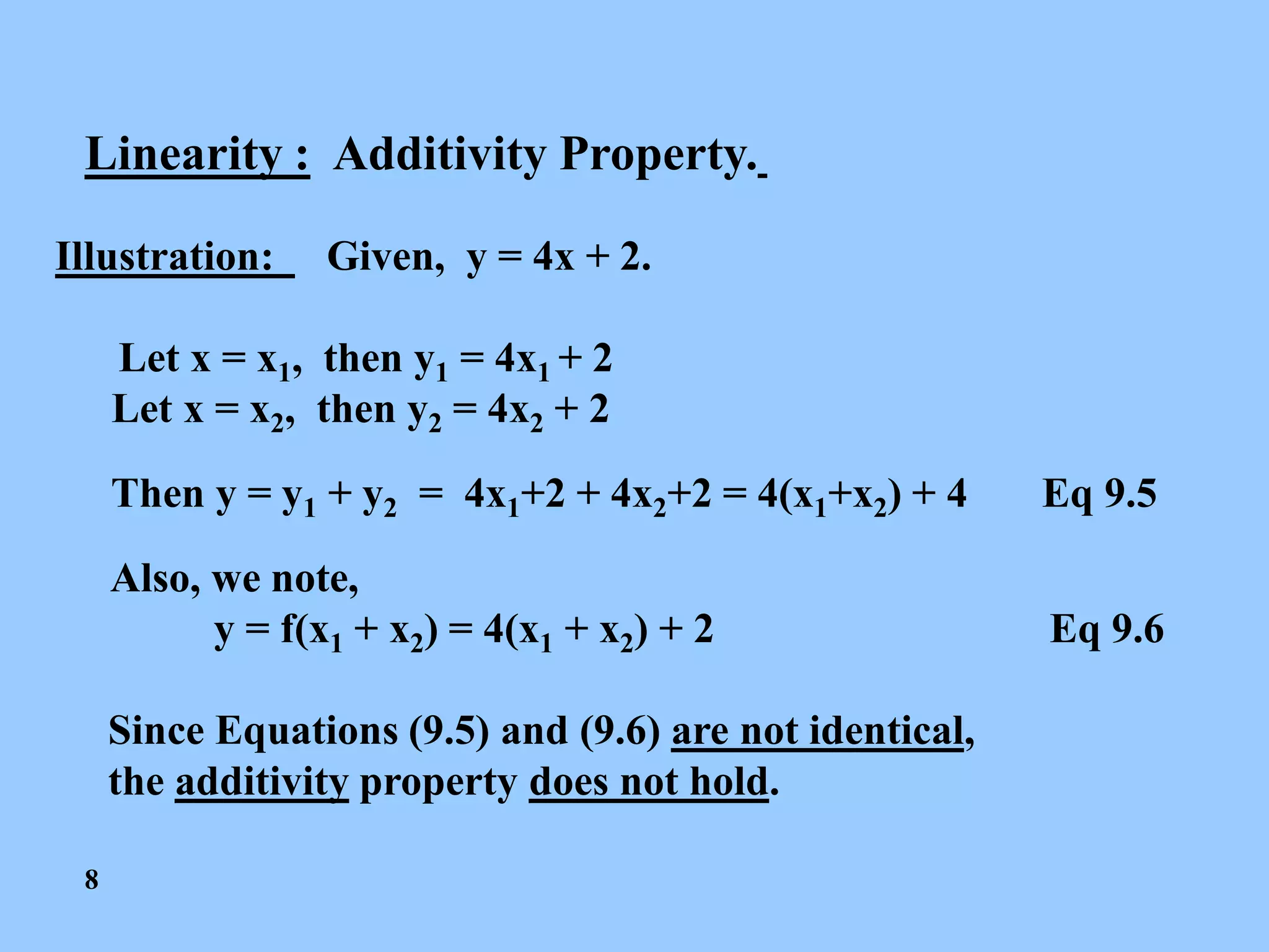
Illustration: Given, y = 4x + 2.
Let x = x1, then y1 = 4x1 + 2
Let x = x2, then y2 = 4x2 + 2
Then y = y1 + y2 = 4x1+2 + 4x2+2 = 4(x1+x2) + 4 Eq 9.5
Also, we note,
y = f(x1 + x2) = 4(x1 + x2) + 2 Eq 9.6
Since Equations (9.5) and (9.6) are not identical,
the additivity property does not hold.
8
Linearity : Example 9.1: Given the circuit shown
in Figure 9.1. Use the concept of linearity
(homogeneity or scaling) to find the current I0.
6  12 
11 
90 V +
_
I0
VS =
Figure 9.1: Circuit for Example 9.1.
Assume I0 = 1 A. Work back to find that this gives
VS = 45 V. But since VS = 90 V this means the true
I0 = 2 A.
9
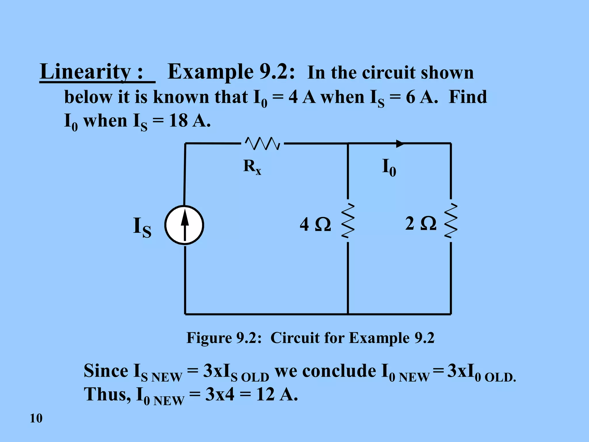
Linearity : Example 9.2: In the circuit shown
below it is known that I0 = 4 A when IS = 6 A. Find
I0 when IS = 18 A.
4  2 
Rx I0
IS
Figure 9.2: Circuit for Example 9.2
Since IS NEW = 3xIS OLD we conclude I0 NEW = 3xI0 OLD.
Thus, I0 NEW = 3x4 = 12 A.
10
Linearity : Question.
For Example 9.2, one might ask, “how do we know the
circuit is linear?” That is a good question. To answer,
we assume a circuit of the same form and determine if we
get a linear equation between the output current and the
input current. What must be shown for the circuit below?
RX
R1 R2
I0
IS
Figure 9.3: Circuit for investigating linearity.
Linearity : Question, continued.
We use the current splitting rule (current division)
to write the following equation.
1
0
1 2
( )( )
( )( )
( )
S
s
I R
I K I
R R
 

Eq 9.7
The equation is of the same form of y = mx, which
we saw was linear. Therefore, if R1 and R2 are constants
then the circuit is linear.
12
15
Superposition Principle
Because the circuit is linear we can find the response of the
circuit to each source acting alone, and then add them up to find
the response of the circuit to all sources acting together. This is
known as the superposition principle.
The superposition principle states that the voltage across (or
the current through) an element in a linear circuit is the
algebraic sum of the voltages across (or currents through) that
element due to each independent source acting alone.
16
Turning sources off
a
b
s
i
s
i i

Current source:
We replace it by a current
source where 0
s
i 
An open-circuit
Voltage source:
DC
+
-
s
v v

s
v
We replace it by a voltage
source where 0
s
v 
An short-circuit
i
17
Steps in Applying the Superposition Principle
1. Turn off all independent sources except
one. Find the output (voltage or current)
due to the active source.
2. Repeat step 1 for each of the other
independent sources.
3. Find the total output by adding
algebraically all of the results found in
steps 1 & 2 above.
Basic Electric Circuits
Superposition: Characterization of Superposition.
Let inputs f1 and f2 be applied to a system y such that,
y = k1f1 + k2f2
Where k1 and k2 are constants of the systems.
Let f1 act alone so that, y = y1 = k1f1
Let f2 act alone so that, y = y2 = k2f2
The property of superposition states that if f1 and f2
Are applied together, the output y will be,
y = y1 + y2 = k1f1 + k2f2
13
Basic Electric Circuits
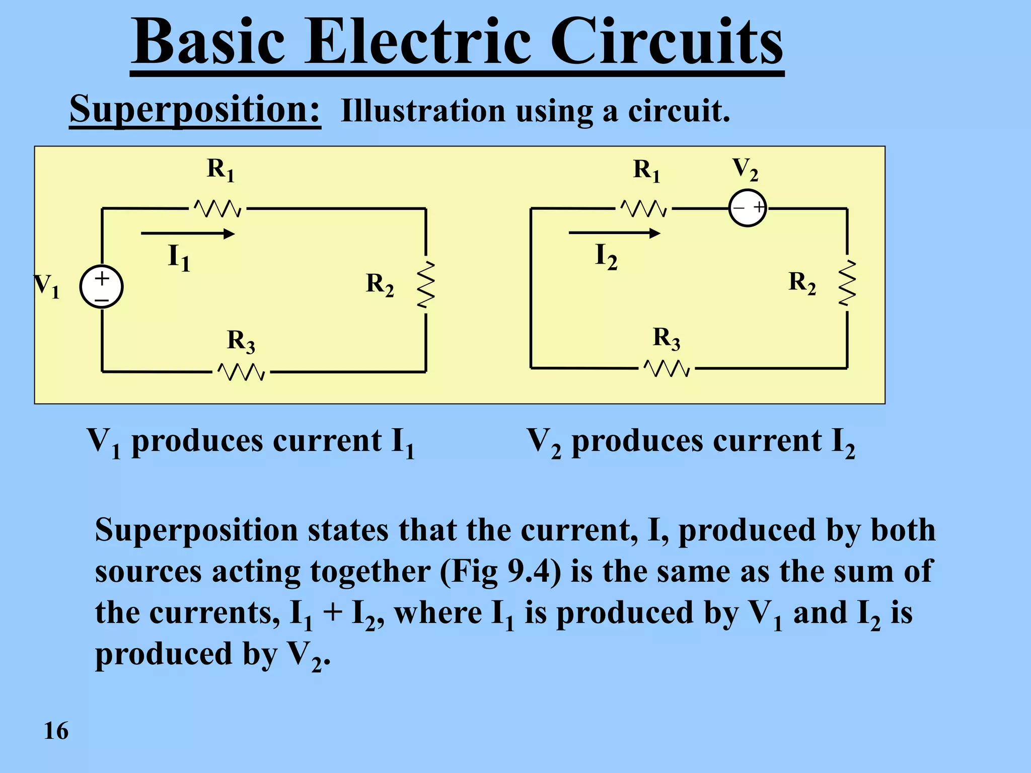
Superposition: Illustration using a circuit.
Consider the circuit below that contains two voltage sources.
V1
V2
R1
R2
R3
+
+
_
_
I
Figure 9.4: Circuit to illustrate superposition
We assume that V1and V2 acting together
produce current I.
15
Basic Electric Circuits
Superposition: Illustration using a circuit.
V1
R1
R2
R3
+
_
I1
V2
R1
R2
R3
I2
+
_
V1 produces current I1 V2 produces current I2
Superposition states that the current, I, produced by both
sources acting together (Fig 9.4) is the same as the sum of
the currents, I1 + I2, where I1 is produced by V1 and I2 is
produced by V2.
16
Basic Electric Circuits
Superposition: Example 9.3. Given the circuit below.
Demonstration by solution that superposition holds.
2  3 
VA
VB
VC
+
+
+
_
_
_
VA = 10 V, VB = 5 V, VC = 15 V
IT
Figure 9.5: Circuit for Example 9.3
With all sources acting: IL = 6 A
17
Basic Electric Circuits
Superposition: Example 9.3. Given the circuit below.
Demonstration by solution that superposition holds.
2  3 
VA
VB
VC
+
+
+
_
_
_
VA = 10 V, VB = 5 V, VC = 15 V
IT
With VA + VB acting, VC = 0: IA+B = 3 A
,
With VC acting, VA + VB = 0: IC = 3 A
We see that superposition holds.
18
Basic Electric Circuits
Superposition: Example 9.4. Given the circuit below.
Find the current I by using superposition.
I
6  VS = 54 V
IS = 3 A
12 
+
_
Figure 9.5: Circuit for Example 9.4.
First, deactivate the source IS and find I in the 6  resistor.
Second, deactivate the source VS and find I in the 6  resistor.
Sum the two currents for the total current.
19
Basic Electric Circuits
Superposition: Example 9.4. Given the circuit below.
Find the current I by using superposition.
IVs
6  VS = 54 V
12 
+
_
IVs = 3 A
20
Basic Electric Circuits
Superposition: Example 9.4. Given the circuit below.
Find the current I by using superposition.
Is
6 
IS = 3 A
12 
3 12
2
(3 12)
S
x
I A
 

Total current I: I = IS + Ivs = 5 A
21
26
Thevenin's Theorem
Linear
Circuit
+
-
V
Variable
R
b
a
In many applications we want to find the response to a particular
element which may, at least at the design stage, be variable.
Each time the variable element
changes we have to re-analyze the
entire circuit. To avoid this we
would like to have a technique that
replaces the linear circuit by
something simple that facilitates the
analysis.
A good approach would be to have a simple equivalent circuit to
replace everything in the circuit except for the variable part (the load).
27
Thevenin's Theorem
Thevenin’s theorem states that a linear two-terminal resistive
circuit can be replaced by an equivalent circuit consisting of a
voltage source VTh in series with a resistor RTh, where VTh is the
open-circuit voltage at the terminals, and RTh is the input or
equivalent resistance at the terminals when the independent
sources are all turned off.
Linear
Circuit
b
a
in
R
L
R
i
DC
b
a
in
R
L
R
i
Th
R
Th
V
28
Thevenin's Theorem
Linear
Circuit
b
a
in
R
L
R
i
DC
b
a
in
R
L
R
i
Th
R
Th
V
Thevenin’s theorem states that the two circuits given below are
equivalent as seen from the load RL that is the same in both cases.
VTh = Thevenin’s voltage = Vab with RL disconnected (= ) = the
open-circuit voltage = VOC
29
Thevenin's Theorem
Linear
Circuit
b
a
in
R
L
R
i
DC
b
a
in
R
L
R
i
Th
R
Th
V
RTh = Thevenin’s resistance = the input resistance with all
independent sources turned off (voltage sources replaced by short
circuits and current sources replaced by open circuits). This is the
resistance seen at the terminals ab when all independent sources are
turned off.
30
Example
DC
10V
 

a
b
2
10V 5V
2 2
OC Th
v V
  

DC
10V
 

a
b
10 2 10
2.5A
2 3 4
2
3
SC
i   

5
2
2.5
Th
Th
SC
V
R
i
   
DC
a
b
5V
Th
V 
2
Th
R  
 

a
b
2 2
1 2
2 2
Th
R

   


More Related Content

Similar to Lecture 05 superposition.pdf

chp10_1introductionewreqttdreasasasasaqqsasaa .pdf
chp10_1introductionewreqttdreasasasasaqqsasaa .pdfchp10_1introductionewreqttdreasasasasaqqsasaa .pdf
chp10_1introductionewreqttdreasasasasaqqsasaa .pdf
muezgebresilassie36
 
03 The Complex Forcing Function.pptx
03 The Complex Forcing Function.pptx03 The Complex Forcing Function.pptx
03 The Complex Forcing Function.pptx
AwaisAsghar31
 

Similar to Lecture 05 superposition.pdf (20)

BEF 12403 - Week 3 - Circuit Laws.ppt
BEF 12403 - Week 3 - Circuit Laws.pptBEF 12403 - Week 3 - Circuit Laws.ppt
BEF 12403 - Week 3 - Circuit Laws.ppt
 
Electric network theorems
Electric network theoremsElectric network theorems
Electric network theorems
 
Ece4762011 lect11[1]
Ece4762011 lect11[1]Ece4762011 lect11[1]
Ece4762011 lect11[1]
 
chp10_1introductionewreqttdreasasasasaqqsasaa .pdf
chp10_1introductionewreqttdreasasasasaqqsasaa .pdfchp10_1introductionewreqttdreasasasasaqqsasaa .pdf
chp10_1introductionewreqttdreasasasasaqqsasaa .pdf
 
5. Power Flow Analaysis-updated SIMULINK
5. Power Flow Analaysis-updated SIMULINK5. Power Flow Analaysis-updated SIMULINK
5. Power Flow Analaysis-updated SIMULINK
 
Circuitanly
CircuitanlyCircuitanly
Circuitanly
 
Project
ProjectProject
Project
 
RGPV BE Ist SEM BEE104 Unit I
RGPV BE Ist SEM BEE104 Unit IRGPV BE Ist SEM BEE104 Unit I
RGPV BE Ist SEM BEE104 Unit I
 
03 The Complex Forcing Function.pptx
03 The Complex Forcing Function.pptx03 The Complex Forcing Function.pptx
03 The Complex Forcing Function.pptx
 
Chapter 1 techniques of dc circuit analysis
Chapter 1 techniques of dc circuit analysisChapter 1 techniques of dc circuit analysis
Chapter 1 techniques of dc circuit analysis
 
Topic 1 b_basic_concepts_and_theorem
Topic 1 b_basic_concepts_and_theoremTopic 1 b_basic_concepts_and_theorem
Topic 1 b_basic_concepts_and_theorem
 
4- Ch04- Circuit Theorems-Sadiku
4- Ch04- Circuit Theorems-Sadiku4- Ch04- Circuit Theorems-Sadiku
4- Ch04- Circuit Theorems-Sadiku
 
Assignmentl3 solutions
Assignmentl3 solutionsAssignmentl3 solutions
Assignmentl3 solutions
 
Electrical and Electronics Engineering
Electrical and Electronics EngineeringElectrical and Electronics Engineering
Electrical and Electronics Engineering
 
Charge Quantization and Magnetic Monopoles
Charge Quantization and Magnetic MonopolesCharge Quantization and Magnetic Monopoles
Charge Quantization and Magnetic Monopoles
 
Basic Electrical Engineering Module 1 Part 1
Basic Electrical Engineering Module 1 Part 1Basic Electrical Engineering Module 1 Part 1
Basic Electrical Engineering Module 1 Part 1
 
Lecture 10
Lecture 10Lecture 10
Lecture 10
 
Electricity lecuture
Electricity lecutureElectricity lecuture
Electricity lecuture
 
Circuit Theory- (Electronics)
Circuit Theory- (Electronics)Circuit Theory- (Electronics)
Circuit Theory- (Electronics)
 
BEEE-UNIT 1.pptx
BEEE-UNIT 1.pptxBEEE-UNIT 1.pptx
BEEE-UNIT 1.pptx
 

Recently uploaded

Future Visions: Predictions to Guide and Time Tech Innovation, Peter Udo Diehl
Future Visions: Predictions to Guide and Time Tech Innovation, Peter Udo DiehlFuture Visions: Predictions to Guide and Time Tech Innovation, Peter Udo Diehl
Future Visions: Predictions to Guide and Time Tech Innovation, Peter Udo Diehl
Peter Udo Diehl
 

Recently uploaded (20)

Future Visions: Predictions to Guide and Time Tech Innovation, Peter Udo Diehl
Future Visions: Predictions to Guide and Time Tech Innovation, Peter Udo DiehlFuture Visions: Predictions to Guide and Time Tech Innovation, Peter Udo Diehl
Future Visions: Predictions to Guide and Time Tech Innovation, Peter Udo Diehl
 
Powerful Start- the Key to Project Success, Barbara Laskowska
Powerful Start- the Key to Project Success, Barbara LaskowskaPowerful Start- the Key to Project Success, Barbara Laskowska
Powerful Start- the Key to Project Success, Barbara Laskowska
 
Measures in SQL (a talk at SF Distributed Systems meetup, 2024-05-22)
Measures in SQL (a talk at SF Distributed Systems meetup, 2024-05-22)Measures in SQL (a talk at SF Distributed Systems meetup, 2024-05-22)
Measures in SQL (a talk at SF Distributed Systems meetup, 2024-05-22)
 
JMeter webinar - integration with InfluxDB and Grafana
JMeter webinar - integration with InfluxDB and GrafanaJMeter webinar - integration with InfluxDB and Grafana
JMeter webinar - integration with InfluxDB and Grafana
 
Designing Great Products: The Power of Design and Leadership by Chief Designe...
Designing Great Products: The Power of Design and Leadership by Chief Designe...Designing Great Products: The Power of Design and Leadership by Chief Designe...
Designing Great Products: The Power of Design and Leadership by Chief Designe...
 
GenAISummit 2024 May 28 Sri Ambati Keynote: AGI Belongs to The Community in O...
GenAISummit 2024 May 28 Sri Ambati Keynote: AGI Belongs to The Community in O...GenAISummit 2024 May 28 Sri Ambati Keynote: AGI Belongs to The Community in O...
GenAISummit 2024 May 28 Sri Ambati Keynote: AGI Belongs to The Community in O...
 
In-Depth Performance Testing Guide for IT Professionals
In-Depth Performance Testing Guide for IT ProfessionalsIn-Depth Performance Testing Guide for IT Professionals
In-Depth Performance Testing Guide for IT Professionals
 
Salesforce Adoption – Metrics, Methods, and Motivation, Antone Kom
Salesforce Adoption – Metrics, Methods, and Motivation, Antone KomSalesforce Adoption – Metrics, Methods, and Motivation, Antone Kom
Salesforce Adoption – Metrics, Methods, and Motivation, Antone Kom
 
10 Differences between Sales Cloud and CPQ, Blanka Doktorová
10 Differences between Sales Cloud and CPQ, Blanka Doktorová10 Differences between Sales Cloud and CPQ, Blanka Doktorová
10 Differences between Sales Cloud and CPQ, Blanka Doktorová
 
IoT Analytics Company Presentation May 2024
IoT Analytics Company Presentation May 2024IoT Analytics Company Presentation May 2024
IoT Analytics Company Presentation May 2024
 
Bits & Pixels using AI for Good.........
Bits & Pixels using AI for Good.........Bits & Pixels using AI for Good.........
Bits & Pixels using AI for Good.........
 
Key Trends Shaping the Future of Infrastructure.pdf
Key Trends Shaping the Future of Infrastructure.pdfKey Trends Shaping the Future of Infrastructure.pdf
Key Trends Shaping the Future of Infrastructure.pdf
 
Exploring UiPath Orchestrator API: updates and limits in 2024 🚀
Exploring UiPath Orchestrator API: updates and limits in 2024 🚀Exploring UiPath Orchestrator API: updates and limits in 2024 🚀
Exploring UiPath Orchestrator API: updates and limits in 2024 🚀
 
How world-class product teams are winning in the AI era by CEO and Founder, P...
How world-class product teams are winning in the AI era by CEO and Founder, P...How world-class product teams are winning in the AI era by CEO and Founder, P...
How world-class product teams are winning in the AI era by CEO and Founder, P...
 
Introduction to Open Source RAG and RAG Evaluation
Introduction to Open Source RAG and RAG EvaluationIntroduction to Open Source RAG and RAG Evaluation
Introduction to Open Source RAG and RAG Evaluation
 
Optimizing NoSQL Performance Through Observability
Optimizing NoSQL Performance Through ObservabilityOptimizing NoSQL Performance Through Observability
Optimizing NoSQL Performance Through Observability
 
Integrating Telephony Systems with Salesforce: Insights and Considerations, B...
Integrating Telephony Systems with Salesforce: Insights and Considerations, B...Integrating Telephony Systems with Salesforce: Insights and Considerations, B...
Integrating Telephony Systems with Salesforce: Insights and Considerations, B...
 
Speed Wins: From Kafka to APIs in Minutes
Speed Wins: From Kafka to APIs in MinutesSpeed Wins: From Kafka to APIs in Minutes
Speed Wins: From Kafka to APIs in Minutes
 
ODC, Data Fabric and Architecture User Group
ODC, Data Fabric and Architecture User GroupODC, Data Fabric and Architecture User Group
ODC, Data Fabric and Architecture User Group
 
Software Delivery At the Speed of AI: Inflectra Invests In AI-Powered Quality
Software Delivery At the Speed of AI: Inflectra Invests In AI-Powered QualitySoftware Delivery At the Speed of AI: Inflectra Invests In AI-Powered Quality
Software Delivery At the Speed of AI: Inflectra Invests In AI-Powered Quality
 

Lecture 05 superposition.pdf

  • 2. 2 Linear Circuits • A linear circuit is one whose output is directly proportional to its input. • Linear circuits obey both the properties of homogeneity (scaling) and additivity.
  • 3. Linearity and Superposition: Linearity. Basically, a mathematical equation is said to be linear if the following properties hold. • homogenity • additivity What does this mean? We first look at the property of homogenity. 1
  • 4. Linearity : Homogeneity. Homogenity requires that if the input (excitation) of a system (equation) is multiplied by a constant, then the output should be obtained by multiplying by the same constant to obtain the correct solution. Sometimes equations that we think are linear, turn out not be be linear because they fail the homogenity property. 2
  • 5. Linearity : Homogeneity (scaling). Illustration: Does homogenity hold for the following equation? Given, y = 4x Eq 9.1 If x = 1, y = 4. If we double x to x = 2 and substitute this value into Eq 9.1 we get y = 8. Now for homogenity to hold, scaling should hold for y. that is, y has a value of 4 when x = 1. If we increase x by a factor of 2 when we should be able to multiply y by the same factor and get the same answer and when we substitute into the right side of the equation for x = 2. 3
  • 6. Linearity : Homogeneity (scaling). Illustration: Does homogenity hold for the following equation? Given, y = 4x + 2 Eq 9.2 If x = 1, then y = 6. If we double x to x=2, then y = 10. Now, since we doubled x we should be able to double the value that y had when x = 1 and get y = 10. In this case we get y = (2)(6) = 12, which obviously is not 10, so homogenity does not hold. We conclude that Eq 9.2 is not a linear equation. In some ways that goes against the gain of what we have been taught about linear equations. 4
  • 7. Linearity : Homogeneity (scaling). y y x x 0 0 2 homogenity holds homogenity does not hold Lnear Not Linear Many of us were brought-up to think that if plotting an equation yields a straight line, then the equation is linear. From the following illustrations we have; 5
  • 8. Linearity : Additivity Property. The additivity property is equivalent to the statement that the response of a system to a sum of inputs is the same as the responses of the system when each input is applied separately and the individual responses summed (added together). This can be explained by considering the following illustrations. 6
  • 9. Linearity : Additivity Property. Illustration: Given, y = 4x. Let x = x1, then y1 = 4x1 Let x = x2, then y2 = 4x2 Then y = y1 + y2 = 4x1 + 4x2 Eq 9.3 Also, we note, y = f(x1 + x2) = 4(x1 + x2) = 4x1 + 4x2 Eq 9.4 Since Equations (9.3) and (9.4) are identical, the additivity property holds. 7
  • 10. Linearity : Additivity Property. Illustration: Given, y = 4x + 2. Let x = x1, then y1 = 4x1 + 2 Let x = x2, then y2 = 4x2 + 2 Then y = y1 + y2 = 4x1+2 + 4x2+2 = 4(x1+x2) + 4 Eq 9.5 Also, we note, y = f(x1 + x2) = 4(x1 + x2) + 2 Eq 9.6 Since Equations (9.5) and (9.6) are not identical, the additivity property does not hold. 8
  • 11. Linearity : Example 9.1: Given the circuit shown in Figure 9.1. Use the concept of linearity (homogeneity or scaling) to find the current I0. 6  12  11  90 V + _ I0 VS = Figure 9.1: Circuit for Example 9.1. Assume I0 = 1 A. Work back to find that this gives VS = 45 V. But since VS = 90 V this means the true I0 = 2 A. 9
  • 12. Linearity : Example 9.2: In the circuit shown below it is known that I0 = 4 A when IS = 6 A. Find I0 when IS = 18 A. 4  2  Rx I0 IS Figure 9.2: Circuit for Example 9.2 Since IS NEW = 3xIS OLD we conclude I0 NEW = 3xI0 OLD. Thus, I0 NEW = 3x4 = 12 A. 10
  • 13. Linearity : Question. For Example 9.2, one might ask, “how do we know the circuit is linear?” That is a good question. To answer, we assume a circuit of the same form and determine if we get a linear equation between the output current and the input current. What must be shown for the circuit below? RX R1 R2 I0 IS Figure 9.3: Circuit for investigating linearity.
  • 14. Linearity : Question, continued. We use the current splitting rule (current division) to write the following equation. 1 0 1 2 ( )( ) ( )( ) ( ) S s I R I K I R R    Eq 9.7 The equation is of the same form of y = mx, which we saw was linear. Therefore, if R1 and R2 are constants then the circuit is linear. 12
  • 15. 15 Superposition Principle Because the circuit is linear we can find the response of the circuit to each source acting alone, and then add them up to find the response of the circuit to all sources acting together. This is known as the superposition principle. The superposition principle states that the voltage across (or the current through) an element in a linear circuit is the algebraic sum of the voltages across (or currents through) that element due to each independent source acting alone.
  • 16. 16 Turning sources off a b s i s i i  Current source: We replace it by a current source where 0 s i  An open-circuit Voltage source: DC + - s v v  s v We replace it by a voltage source where 0 s v  An short-circuit i
  • 17. 17 Steps in Applying the Superposition Principle 1. Turn off all independent sources except one. Find the output (voltage or current) due to the active source. 2. Repeat step 1 for each of the other independent sources. 3. Find the total output by adding algebraically all of the results found in steps 1 & 2 above.
  • 18. Basic Electric Circuits Superposition: Characterization of Superposition. Let inputs f1 and f2 be applied to a system y such that, y = k1f1 + k2f2 Where k1 and k2 are constants of the systems. Let f1 act alone so that, y = y1 = k1f1 Let f2 act alone so that, y = y2 = k2f2 The property of superposition states that if f1 and f2 Are applied together, the output y will be, y = y1 + y2 = k1f1 + k2f2 13
  • 19. Basic Electric Circuits Superposition: Illustration using a circuit. Consider the circuit below that contains two voltage sources. V1 V2 R1 R2 R3 + + _ _ I Figure 9.4: Circuit to illustrate superposition We assume that V1and V2 acting together produce current I. 15
  • 20. Basic Electric Circuits Superposition: Illustration using a circuit. V1 R1 R2 R3 + _ I1 V2 R1 R2 R3 I2 + _ V1 produces current I1 V2 produces current I2 Superposition states that the current, I, produced by both sources acting together (Fig 9.4) is the same as the sum of the currents, I1 + I2, where I1 is produced by V1 and I2 is produced by V2. 16
  • 21. Basic Electric Circuits Superposition: Example 9.3. Given the circuit below. Demonstration by solution that superposition holds. 2  3  VA VB VC + + + _ _ _ VA = 10 V, VB = 5 V, VC = 15 V IT Figure 9.5: Circuit for Example 9.3 With all sources acting: IL = 6 A 17
  • 22. Basic Electric Circuits Superposition: Example 9.3. Given the circuit below. Demonstration by solution that superposition holds. 2  3  VA VB VC + + + _ _ _ VA = 10 V, VB = 5 V, VC = 15 V IT With VA + VB acting, VC = 0: IA+B = 3 A , With VC acting, VA + VB = 0: IC = 3 A We see that superposition holds. 18
  • 23. Basic Electric Circuits Superposition: Example 9.4. Given the circuit below. Find the current I by using superposition. I 6  VS = 54 V IS = 3 A 12  + _ Figure 9.5: Circuit for Example 9.4. First, deactivate the source IS and find I in the 6  resistor. Second, deactivate the source VS and find I in the 6  resistor. Sum the two currents for the total current. 19
  • 24. Basic Electric Circuits Superposition: Example 9.4. Given the circuit below. Find the current I by using superposition. IVs 6  VS = 54 V 12  + _ IVs = 3 A 20
  • 25. Basic Electric Circuits Superposition: Example 9.4. Given the circuit below. Find the current I by using superposition. Is 6  IS = 3 A 12  3 12 2 (3 12) S x I A    Total current I: I = IS + Ivs = 5 A 21
  • 26. 26 Thevenin's Theorem Linear Circuit + - V Variable R b a In many applications we want to find the response to a particular element which may, at least at the design stage, be variable. Each time the variable element changes we have to re-analyze the entire circuit. To avoid this we would like to have a technique that replaces the linear circuit by something simple that facilitates the analysis. A good approach would be to have a simple equivalent circuit to replace everything in the circuit except for the variable part (the load).
  • 27. 27 Thevenin's Theorem Thevenin’s theorem states that a linear two-terminal resistive circuit can be replaced by an equivalent circuit consisting of a voltage source VTh in series with a resistor RTh, where VTh is the open-circuit voltage at the terminals, and RTh is the input or equivalent resistance at the terminals when the independent sources are all turned off. Linear Circuit b a in R L R i DC b a in R L R i Th R Th V
  • 28. 28 Thevenin's Theorem Linear Circuit b a in R L R i DC b a in R L R i Th R Th V Thevenin’s theorem states that the two circuits given below are equivalent as seen from the load RL that is the same in both cases. VTh = Thevenin’s voltage = Vab with RL disconnected (= ) = the open-circuit voltage = VOC
  • 29. 29 Thevenin's Theorem Linear Circuit b a in R L R i DC b a in R L R i Th R Th V RTh = Thevenin’s resistance = the input resistance with all independent sources turned off (voltage sources replaced by short circuits and current sources replaced by open circuits). This is the resistance seen at the terminals ab when all independent sources are turned off.
  • 30. 30 Example DC 10V    a b 2 10V 5V 2 2 OC Th v V     DC 10V    a b 10 2 10 2.5A 2 3 4 2 3 SC i     5 2 2.5 Th Th SC V R i     DC a b 5V Th V  2 Th R      a b 2 2 1 2 2 2 Th R      