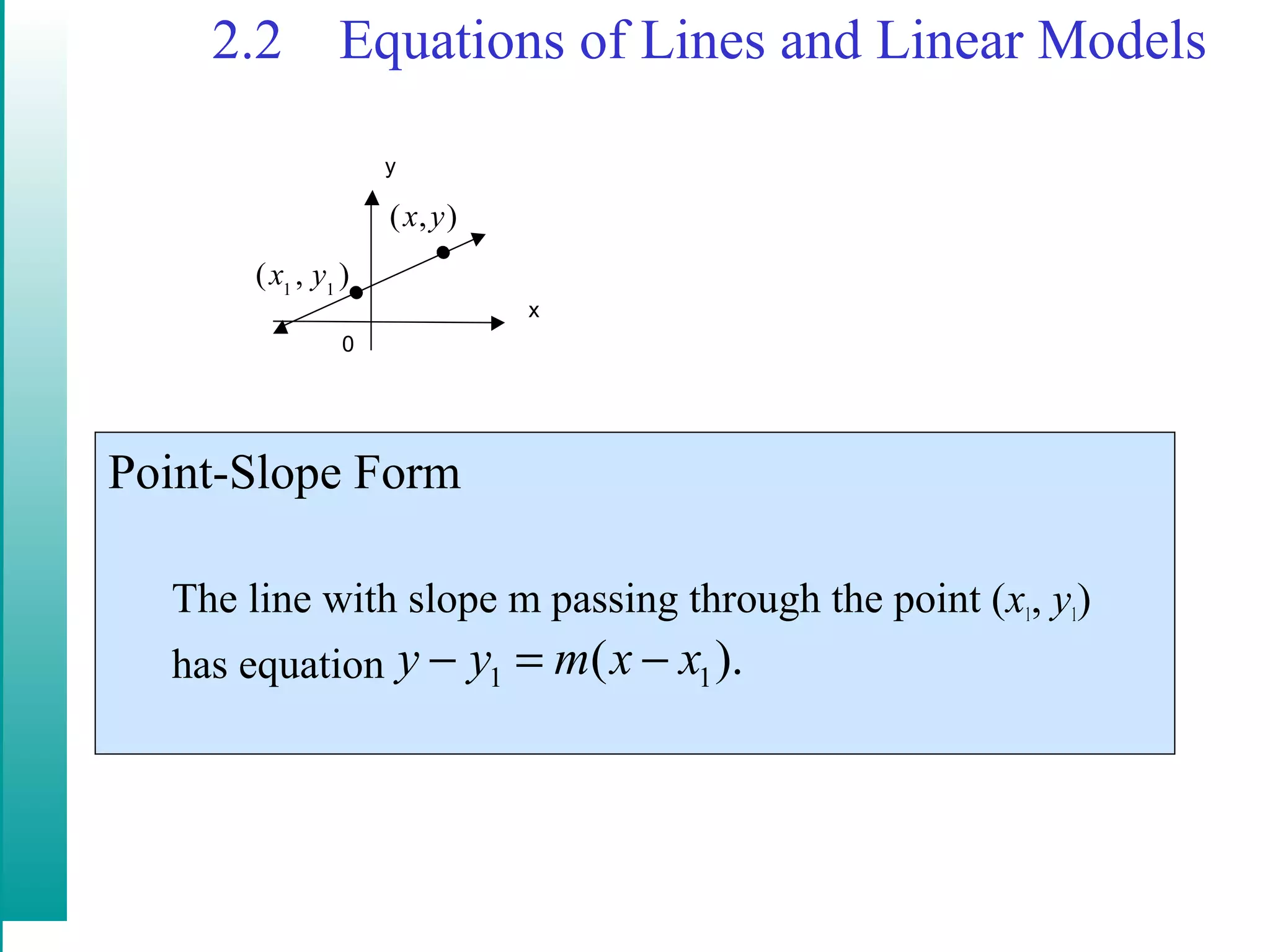
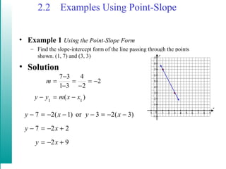
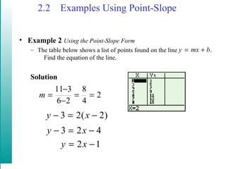
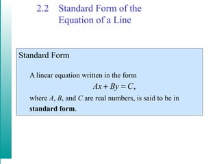
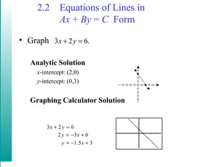
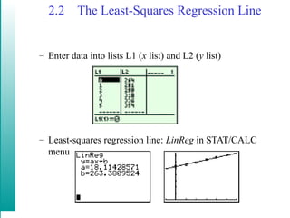
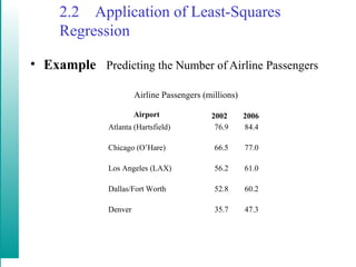
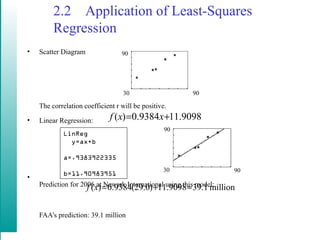
2.2 Equations of Lines and Linear Models
Point-Slope Form
The line with slope m passing through the point (x1, y1)
has equation
x
y
0
),( yx
),( 11
yx
1 1( ).y y m x x− = −
2.2 Examples Using Point-Slope
• Example 1 Using the Point-Slope Form
– Find the slope-intercept form of the line passing through the points
shown. (1, 7) and (3, 3)
• Solution
)(
2
2
4
31
37
11
xxmyy
m
−=−
−=
−
=
−
−
=
92
227
)3(23or)1(27
+−=
+−=−
−−=−−−=−
xy
xy
xyxy
2.2 Examples Using Point-Slope
• Example 2 Using the Point-Slope Form
– The table below shows a list of points found on the line
Find the equation of the line.
Solution
.bmxy +=
2
4
8
26
311
==
−
−
=m
)2(23 −=− xy
423 −=− xy
12 −= xy
2.2 Standard Form of the
Equation of a Line
Standard Form
A linear equation written in the form
where A, B, and C are real numbers, is said to be in
standard form.
,Ax By C+ =
2.2 Equations of Lines in
Ax + By = C Form
• Graph
Analytic Solution
x-intercept: (2,0)
y-intercept: (0,3)
Graphing Calculator Solution
.623 =+ yx
623 =+ yx
632 +−= xy
35.1 +−= xy
2.2 Parallel Lines
Parallel Lines
Two distinct nonvertical lines are parallel if and
only if they have the same slope.
2.2 Parallel Lines
Example
Find the equation of the line that passes through the point (3,5)
and is parallel to the line with equation Graph
both lines in the standard viewing window.
Solution
.452 =+ yx
5
4
5
2
452
+−=
=+
xy
yx Solve for y in
terms of x.
5
2
slope −=m
2.2 Parallel Lines
5
31
5
2
3125
62255
)3(2)5(5
)3(
5
2
5
)( 11
+−=
+−=
+−=−
−−=−
−−=−
−=−
xy
xy
xy
xy
xy
xxmyy
10-10
-10
10
5
4
5
2
+−= xy
5
31
5
2
+−= xy
2.2 Perpendicular Lines
Perpendicular Lines
Two lines, neither of which is vertical, are
perpendicular if and only if their slopes have
product –1.
2.2 Perpendicular Lines
Example Find the equation of the line that passes through the point
(3,5) and is perpendicular to the line with equation
Graph both lines in the standard viewing window.
Use slope from the previous example.
The slope of a perpendicular line is
.452 =+ yx
5
2
−=m
.
2
5
=m
5
5 ( 3)
2
2( 5) 5( 3)
2 10 5 15
2 5 5
5 5
2 2
y x
y x
y x
y x
y x
− = −
− = −
− = −
= −
= −
2.2 Perpendicular Lines
-15
10
-10
15
5 5
2 2y x= −
2 4
5 5y x= − +
2.2 Modeling Medicare Costs
• Linear Models and Regression
– Discrete data points can be plotted and the graph is
called a scatter diagram.
– Useful when analyzing trends in data.
– e.g. Estimates for Medicare costs (in billions)
x (Year) y (Cost)
2002 264
2003 281
2004 299
2005 318
2006 336
2007 354
2.2 Modeling Medicare Costs
a) Scatter diagram where x = 0 corresponds to 2002, x = 1 to 2003, etc.
Data points (0, 264), (1, 281), (2, 299),
(3, 318), (4, 336) and (5, 354)
b) Linear model – pick 2 points,
(0, 264) and (3, 318)
c) Predict cost of Medicare in 2010.
318 264
18, with -intercept (0, 264)
3 0
We have the line ( ) 18 264
m y
f x x
−
= =
−
= +
(8) 18(8) 264 408
Prediction- Medicare costs will reach $408 billion in 2010.
f = + =
2.2 The Least-Squares Regression Line
– Enter data into lists L1 (x list) and L2 (y list)
– Least-squares regression line: LinReg in STAT/CALC
menu
2.2 Correlation Coefficient
• Correlation Coefficient r
– Determines if a linear model is appropriate
• range of r:
• r near +1, low x-values correspond to low y-values
and high x-values correspond to high y-values.
• r near –1, low x-values correspond to high y-values
and high x-values correspond to low y-values.
• means there is little or no correlation.
– To calculate r using the TI-83, turn
Diagnostic On in the Catalog menu.
11 ≤≤− r
0≈r
2.2 Application of Least-Squares
Regression
• Example Predicting the Number of Airline Passengers
Atlanta (Hartsfield) 76.9 84.4
Chicago (O’Hare) 66.5 77.0
Los Angeles (LAX) 56.2 61.0
Dallas/Fort Worth 52.8 60.2
Denver 35.7 47.3
Airline Passengers (millions)
2002 2006Airport
2.2 Application of Least-Squares
Regression
• Scatter Diagram
The correlation coefficient r will be positive.
• Linear Regression:
•
Prediction for 2006 at Newark International using this model:
FAA’s prediction: 39.1 million
30
90
90
90
90
30
( ) 0.9384 11.9098f x x= +
( ) 0.9384(29.0) 11.9098 39.1 millionf x = + ≈
LinReg
y=ax+b
a=.9383922335
b=11.90983951

Math Section 2.2 ECC Etudes

  • 1.
    2.2 Equations ofLines and Linear Models Point-Slope Form The line with slope m passing through the point (x1, y1) has equation x y 0 ),( yx ),( 11 yx 1 1( ).y y m x x− = −
  • 2.
    2.2 Examples UsingPoint-Slope • Example 1 Using the Point-Slope Form – Find the slope-intercept form of the line passing through the points shown. (1, 7) and (3, 3) • Solution )( 2 2 4 31 37 11 xxmyy m −=− −= − = − − = 92 227 )3(23or)1(27 +−= +−=− −−=−−−=− xy xy xyxy
  • 3.
    2.2 Examples UsingPoint-Slope • Example 2 Using the Point-Slope Form – The table below shows a list of points found on the line Find the equation of the line. Solution .bmxy += 2 4 8 26 311 == − − =m )2(23 −=− xy 423 −=− xy 12 −= xy
  • 4.
    2.2 Standard Formof the Equation of a Line Standard Form A linear equation written in the form where A, B, and C are real numbers, is said to be in standard form. ,Ax By C+ =
  • 5.
    2.2 Equations ofLines in Ax + By = C Form • Graph Analytic Solution x-intercept: (2,0) y-intercept: (0,3) Graphing Calculator Solution .623 =+ yx 623 =+ yx 632 +−= xy 35.1 +−= xy
  • 6.
    2.2 Parallel Lines ParallelLines Two distinct nonvertical lines are parallel if and only if they have the same slope.
  • 7.
    2.2 Parallel Lines Example Findthe equation of the line that passes through the point (3,5) and is parallel to the line with equation Graph both lines in the standard viewing window. Solution .452 =+ yx 5 4 5 2 452 +−= =+ xy yx Solve for y in terms of x. 5 2 slope −=m
  • 8.
    2.2 Parallel Lines 5 31 5 2 3125 62255 )3(2)5(5 )3( 5 2 5 )(11 +−= +−= +−=− −−=− −−=− −=− xy xy xy xy xy xxmyy 10-10 -10 10 5 4 5 2 +−= xy 5 31 5 2 +−= xy
  • 9.
    2.2 Perpendicular Lines PerpendicularLines Two lines, neither of which is vertical, are perpendicular if and only if their slopes have product –1.
  • 10.
    2.2 Perpendicular Lines ExampleFind the equation of the line that passes through the point (3,5) and is perpendicular to the line with equation Graph both lines in the standard viewing window. Use slope from the previous example. The slope of a perpendicular line is .452 =+ yx 5 2 −=m . 2 5 =m
  • 11.
    5 5 ( 3) 2 2(5) 5( 3) 2 10 5 15 2 5 5 5 5 2 2 y x y x y x y x y x − = − − = − − = − = − = − 2.2 Perpendicular Lines -15 10 -10 15 5 5 2 2y x= − 2 4 5 5y x= − +
  • 12.
    2.2 Modeling MedicareCosts • Linear Models and Regression – Discrete data points can be plotted and the graph is called a scatter diagram. – Useful when analyzing trends in data. – e.g. Estimates for Medicare costs (in billions) x (Year) y (Cost) 2002 264 2003 281 2004 299 2005 318 2006 336 2007 354
  • 13.
    2.2 Modeling MedicareCosts a) Scatter diagram where x = 0 corresponds to 2002, x = 1 to 2003, etc. Data points (0, 264), (1, 281), (2, 299), (3, 318), (4, 336) and (5, 354) b) Linear model – pick 2 points, (0, 264) and (3, 318) c) Predict cost of Medicare in 2010. 318 264 18, with -intercept (0, 264) 3 0 We have the line ( ) 18 264 m y f x x − = = − = + (8) 18(8) 264 408 Prediction- Medicare costs will reach $408 billion in 2010. f = + =
  • 14.
    2.2 The Least-SquaresRegression Line – Enter data into lists L1 (x list) and L2 (y list) – Least-squares regression line: LinReg in STAT/CALC menu
  • 15.
    2.2 Correlation Coefficient •Correlation Coefficient r – Determines if a linear model is appropriate • range of r: • r near +1, low x-values correspond to low y-values and high x-values correspond to high y-values. • r near –1, low x-values correspond to high y-values and high x-values correspond to low y-values. • means there is little or no correlation. – To calculate r using the TI-83, turn Diagnostic On in the Catalog menu. 11 ≤≤− r 0≈r
  • 16.
    2.2 Application ofLeast-Squares Regression • Example Predicting the Number of Airline Passengers Atlanta (Hartsfield) 76.9 84.4 Chicago (O’Hare) 66.5 77.0 Los Angeles (LAX) 56.2 61.0 Dallas/Fort Worth 52.8 60.2 Denver 35.7 47.3 Airline Passengers (millions) 2002 2006Airport
  • 17.
    2.2 Application ofLeast-Squares Regression • Scatter Diagram The correlation coefficient r will be positive. • Linear Regression: • Prediction for 2006 at Newark International using this model: FAA’s prediction: 39.1 million 30 90 90 90 90 30 ( ) 0.9384 11.9098f x x= + ( ) 0.9384(29.0) 11.9098 39.1 millionf x = + ≈ LinReg y=ax+b a=.9383922335 b=11.90983951