1. Ch 7.2: Review of Matrices
For theoretical and computation reasons, we review results
of matrix theory in this section and the next.
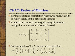
A matrix A is an m x n rectangular array of elements,
arranged in m rows and n columns, denoted
Some examples of 2 x 2 matrices are given below:
( )
==
mnmm
n
n
ji
aaa
aaa
aaa
a
21
22221
11211
A
−+
−
=
=
=
ii
i
CB
7654
231
,
42
31
,
43
21
A
2. Transpose
The transpose of A = (aij) is AT
= (aji).
For example,
=⇒
=
mnnn
m
m
T
mnmm
n
n
aaa
aaa
aaa
aaa
aaa
aaa
21
22212
12111
21
22221
11211
AA
=⇒
=
=⇒
=
63
52
41
654
321
,
42
31
43
21 TT
BBAA
3. Conjugate
The conjugate of A = (aij) is A = (aij).
For example,
=⇒
=
mnmm
n
n
mnmm
n
n
aaa
aaa
aaa
aaa
aaa
aaa
21
22221
11211
21
22221
11211
AA
+
−
=⇒
−
+
=
443
321
443
321
i
i
i
i
AA
4. Adjoint
The adjoint of A is AT
, and is denoted by A*
For example,
=⇒
=
mnnn
m
m
mnmm
n
n
aaa
aaa
aaa
aaa
aaa
aaa
21
22212
12111
*
21
22221
11211
AA
−
+
=⇒
−
+
=
432
431
443
321 *
i
i
i
i
AA
5. Square Matrices
A square matrix A has the same number of rows and
columns. That is, A is n x n. In this case, A is said to have
order n.
For example,
=
nnnn
n
n
aaa
aaa
aaa
21
22221
11211
A
=
=
987
654
321
,
43
21
BA
6. Vectors
A column vector x is an n x 1 matrix. For example,
A row vector x is a 1 x n matrix. For example,
Note here that y = xT
, and that in general, if x is a column
vector x, then xT
is a row vector.
=
3
2
1
x
( )321=y
7. The Zero Matrix
The zero matrix is defined to be 0 = (0), whose dimensions
depend on the context. For example,
,
00
00
00
,
000
000
,
00
00
=
=
= 000
8. Matrix Equality
Two matrices A = (aij) and B = (bij) are equal if aij = bij for
all i and j. For example,
BABA =⇒
=
=
43
21
,
43
21
9. Matrix – Scalar Multiplication
The product of a matrix A = (aij) and a constant k is defined
to be kA = (kaij). For example,
−−−
−−−
=−⇒
=
302520
15105
5
654
321
AA
10. Matrix Addition and Subtraction
The sum of two m x n matrices A = (aij) and B = (bij) is
defined to be A + B = (aij + bij). For example,
The difference of two m x n matrices A = (aij) and B = (bij)
is defined to be A - B = (aij - bij). For example,
=+⇒
=
=
1210
86
87
65
,
43
21
BABA
−−
−−
=−⇒
=
=
44
44
87
65
,
43
21
BABA
11. Matrix Multiplication
The product of an m x n matrix A = (aij) and an n x r matrix
B = (bij) is defined to be the matrix C = (cij), where
Examples (note AB does not necessarily equal BA):
∑=
=
n
k
kjikij bac
1
=
−+++
−+++
=⇒
−
=
=
=
++
++
=⇒
=
++
++
=⇒
=
=
417
15
61000512
340023
10
21
03
,
654
321
2014
1410
164122
12291
2511
115
16983
8341
42
31
,
43
21
CDDC
BA
ABBA
12. Vector Multiplication
The dot product of two n x 1 vectors x & y is defined as
The inner product of two n x 1 vectors x & y is defined as
Example:
∑=
=
n
k
ji
T
yx
1
yx
( ) ∑=
==
n
k
ji
T
yx,
1
yxyx
( ) iiii,
iiii
i
i
i
T
T
2118)55)(3()32)(2()1)(1(
912)55)(3()32)(2()1)(1(
55
32
1
,
3
2
1
+=−+++−==⇒
+−=++−+−=⇒
+
−
−
=
=
yxyx
yxyx
13. Vector Length
The length of an n x 1 vector x is defined as
Note here that we have used the fact that if x = a + bi, then
Example:
( )
2/1
1
2
2/1
1
2/1
||
=
== ∑∑ ==
n
k
k
n
k
kk xxx,xxx
( )
( ) 3016941
)43)(43()2)(2()1)(1(
43
2
1
2/1
=+++=
−+++==⇒
+
= ii,
i
xxxx
( )( ) 222
xbabiabiaxx =+=−+=⋅
14. Orthogonality
Two n x 1 vectors x & y are orthogonal if (x,y) = 0.
Example:
( ) 0)1)(3()4)(2()11)(1(
1
4
11
3
2
1
=−+−+=⇒
−
−=
= yxyx ,
15. Identity Matrix
The multiplicative identity matrix I is an n x n matrix
given by
For any square matrix A, it follows that AI = IA = A.
The dimensions of I depend on the context. For example,
=
100
010
001
I
=
=
=
=
987
654
321
987
654
321
100
010
001
,
43
21
10
01
43
21
IBAI
16. Inverse Matrix
A square matrix A is nonsingular, or invertible, if there
exists a matrix B such that that AB = BA = I. Otherwise A
is singular.
The matrix B, if it exists, is unique and is denoted by A-1
and
is called the inverse of A.
It turns out that A-1
exists iff detA ≠ 0, and A-1
can be found
using row reduction (also called Gaussian elimination) on
the augmented matrix (A|I), see example on next slide.
The three elementary row operations:
Interchange two rows.
Multiply a row by a nonzero scalar.
Add a multiple of one row to another row.
17. Example: Finding the Identity Matrix (1 of 2)
Use row reduction to find the inverse of the matrix A below,
if it exists.
Solution: If possible, use elementary row operations to
reduce (A|I),
such that the left side is the identity matrix, for then the
right side will be A-1
. (See next slide.)
−
=
834
301
210
A
( ) ,
100834
010301
001210
−
=IA
19. Matrix Functions
The elements of a matrix can be functions of a real variable.
In this case, we write
Such a matrix is continuous at a point, or on an interval
(a, b), if each element is continuous there. Similarly with
differentiation and integration:
=
=
)()()(
)()()(
)()()(
)(,
)(
)(
)(
)(
21
22221
11211
2
1
tatata
tatata
tatata
t
tx
tx
tx
t
mnmm
n
n
m
Ax
=
= ∫∫
b
a
ij
b
a
ij
dttadtt
dt
da
dt
d
)()(, A
A
20. Example & Differentiation Rules
Example:
Many of the rules from calculus apply in this setting. For
example: ( )
( )
( )
+
=
+=
+
=
dt
d
dt
d
dt
d
dt
d
dt
d
dt
d
dt
d
dt
d
B
AB
AAB
BABA
C
A
C
CA
matrixconstantaiswhere,
−
=⇒
−
=⇒
=
∫ π
ππ
41
0
)(
,
0sin
cos6
4cos
sin3
)(
3
0
2
dtt
t
tt
dt
d
t
tt
t
A
A
A