1. Ch 6.3: Step Functions
Some of the most interesting elementary applications of the
Laplace Transform method occur in the solution of linear
equations with discontinuous or impulsive forcing functions.
In this section, we will assume that all functions considered
are piecewise continuous and of exponential order, so that
their Laplace Transforms all exist, for s large enough.
2. Step Function definition
Let c ≥ 0. The unit step function, or Heaviside function, is
defined by
A negative step can be represented by
≥
<
=
ct
ct
tuc
,1
,0
)(
≥
<
=−=
ct
ct
tuty c
,0
,1
)(1)(
3. Example 1
Sketch the graph of
Solution: Recall that uc(t) is defined by
Thus
and hence the graph of h(t) is a rectangular pulse.
0),()()( 2 ≥−= ttututh ππ
≥
<
=
ct
ct
tuc
,1
,0
)(
∞<≤
<≤
<≤
=
t
t
t
th
π
ππ
π
20
2,1
0,0
)(
4. Laplace Transform of Step Function
The Laplace Transform of uc(t) is
{ }
s
e
s
e
s
e
e
s
dte
dtedttuetuL
cs
csbs
b
b
c
st
b
b
c
st
b
c
st
c
st
c
−
−−
∞→
−
∞→
−
∞→
∞
−
∞
−
=
+−=
−==
==
∫
∫∫
lim
1
limlim
)()(
0
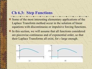
5. Translated Functions
Given a function f (t) defined for t ≥ 0, we will often want to
consider the related function g(t) = uc(t) f (t - c):
Thus g represents a translation of f a distance c in the
positive t direction.
In the figure below, the graph of f is given on the left, and
the graph of g on the right.
≥−
<
=
ctctf
ct
tg
),(
,0
)(
6. Example 2
Sketch the graph of
Solution: Recall that uc(t) is defined by
Thus
and hence the graph of g(t) is a shifted parabola.
.0,)(where),()1()( 2
1 ≥=−= tttftutftg
≥
<
=
ct
ct
tuc
,1
,0
)(
≥−
<≤
=
1,)1(
10,0
)( 2
tt
t
tg
7. Theorem 6.3.1
If F(s) = L{f (t)} exists for s > a ≥ 0, and if c > 0, then
Conversely, if f (t) = L-1
{F(s)}, then
Thus the translation of f (t) a distance c in the positive t
direction corresponds to a multiplication of F(s) by e-cs
.
{ } { } )()()()( sFetfLectftuL cscs
c
−−
==−
{ })()()( 1
sFeLctftu cs
c
−−
=−
8. Theorem 6.3.1: Proof Outline
We need to show
Using the definition of the Laplace Transform, we have
{ }
)(
)(
)(
)(
)()()()(
0
0
)(
0
sFe
duufee
duufe
dtctfe
dtctftuectftuL
cs
sucs
cus
ctu
c
st
c
st
c
−
∞
−−
∞
+−
−=
∞
−
∞
−
=
=
=
−=
−=−
∫
∫
∫
∫
{ } )()()( sFectftuL cs
c
−
=−
9. Example 3
Find the Laplace transform of
Solution: Note that
Thus
)()1()( 1
2
tuttf −=
≥−
<≤
=
1,)1(
10,0
)( 2
tt
t
tf
{ } { } { } 3
22
1
2
)1)(()(
s
e
tLettuLtfL
s
s
−
−
==−=
10. Example 4
Find L{ f (t)}, where f is defined by
Note that f (t) = sin(t) + uπ/4(t) cos(t - π/4), and
≥−+
<≤
=
4/),4/cos(sin
4/0,sin
)(
ππ
π
ttt
tt
tf
{ } { } { }
{ } { }
1
1
11
1
cossin
)4/cos()(sin)(
2
4/
2
4/
2
4/
4/
+
+
=
+
+
+
=
+=
−+=
−
−
−
s
se
s
s
e
s
tLetL
ttuLtLtfL
s
s
s
π
π
π
π π
11. Example 5
Find L-1
{F(s)}, where
Solution:
4
7
3
)(
s
e
sF
s−
+
=
( )3
7
3
4
71
4
1
4
7
1
4
1
7)(
6
1
2
1
!3
6
1!3
2
1
3
)(
−+=
⋅+
=
+
=
−−−
−
−−
ttut
s
eL
s
L
s
e
L
s
Ltf
s
s
12. Theorem 6.3.2
If F(s) = L{f (t)} exists for s > a ≥ 0, and if c is a constant,
then
Conversely, if f (t) = L-1
{F(s)}, then
Thus multiplication f (t) by ect
results in translating F(s) a
distance c in the positive t direction, and conversely.
Proof Outline:
{ } cascsFtfeL ct
+>−= ),()(
{ })()( 1
csFLtfect
−= −
{ } )()()()(
0
)(
0
csFdttfedttfeetfeL tcsctstct
−=== ∫∫
∞
−−
∞
−
13. Example 4
Find the inverse transform of
To solve, we first complete the square:
Since
it follows that
52
1
)( 2
++
+
=
ss
s
sG
( )
( )
( ) 41
1
412
1
52
1
)( 222
++
+
=
+++
+
=
++
+
=
s
s
ss
s
ss
s
sG
{ } { } ( )tetfesFLsGL tt
2cos)()1()( 11 −−−−
==+=
{ } ( )t
s
s
LsFLtf 2cos
4
)()( 2
11
=
+
== −−