1. Ch 6.5: Impulse Functions
In some applications, it is necessary to deal with phenomena
of an impulsive nature.
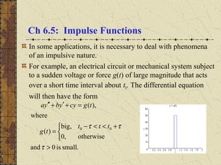
For example, an electrical circuit or mechanical system subject
to a sudden voltage or force g(t) of large magnitude that acts
over a short time interval about t0. The differential equation
will then have the form
small.is0and
otherwise,0
,big
)(
where
),(
00
>
+<<−
=
=+′+′′
τ
ττ ttt
tg
tgcyybya
2. Measuring Impulse
In a mechanical system, where g(t) is a force, the total impulse
of this force is measured by the integral
Note that if g(t) has the form
then
In particular, if c = 1/(2τ), then I(τ) = 1 (independent of τ).
∫∫
+
−
∞
∞−
==
τ
τ
τ
0
0
)()()(
t
t
dttgdttgI
+<<−
=
otherwise,0
,
)( 00 ττ tttc
tg
0,2)()()(
0
0
>=== ∫∫
+
−
∞
∞−
τττ
τ
τ
cdttgdttgI
t
t
3. Unit Impulse Function
Suppose the forcing function dτ(t) has the form
Then as we have seen, I(τ) = 1.
We are interested dτ(t) acting over
shorter and shorter time intervals
(i.e., τ → 0). See graph on right.
Note that dτ(t) gets taller and narrower
as τ → 0. Thus for t ≠ 0, we have
<<−
=
otherwise,0
,21
)(
τττ
τ
t
td
1)(limand,0)(lim
00
==
→→
τ
τ
τ
τ
Itd
4. Dirac Delta Function
Thus for t ≠ 0, we have
The unit impulse function δ is defined to have the properties
The unit impulse function is an example of a generalized
function and is usually called the Dirac delta function.
In general, for a unit impulse at an arbitrary point t0,
1)(limand,0)(lim
00
==
→→
τ
τ
τ
τ
Itd
1)(and,0for0)( =≠= ∫
∞
∞−
dtttt δδ
1)(and,for0)( 000 =−≠=− ∫
∞
∞−
dttttttt δδ
5. Laplace Transform of δ (1 of 2)
The Laplace Transform of δ is defined by
and thus
{ } { } 0,)(lim)( 00
0
0 >−=−
→
tttdLttL τ
τ
δ
{ }
( ) ( )
[ ]
00
0
0
00
0
0
0
0
)cosh(
lim
)sinh(
lim
2
lim
2
1
lim
2
lim
2
1
lim)(lim)(
0
00
00
00
0
0
0
stst
st
ssst
tsts
t
t
st
t
t
stst
e
s
ss
e
s
s
e
ee
s
e
ee
ss
e
dtedtttdettL
−
→
−
→
−
−−
→
−−+−
→
+
−
−
→
+
−
−
→
∞
−
→
=
=
=
−
=
+−=
−
=
=−=− ∫∫
τ
τ
τ
τ
ττ
τ
δ
τ
τ
ττ
τ
ττ
τ
τ
τ
τ
τ
ττ
τ
τ
6. Laplace Transform of δ (2 of 2)
Thus the Laplace Transform of δ is
For Laplace Transform of δ at t0= 0, take limit as follows:
For example, when t0= 10, we have L{δ(t-10)} = e-10s
.
{ } 0,)( 00
0
>=− −
tettL st
δ
{ } { } 1lim)(lim)( 0
00 0
0
0
==−= −
→→
st
t
ettdLtL
τ
τδ
7. Product of Continuous Functions and δ
The product of the delta function and a continuous function f
can be integrated, using the mean value theorem for integrals:
Thus
[ ]
)(
*)(lim
)*where(*)(2
2
1
lim
)(
2
1
lim
)()(lim)()(
0
0
00
0
0
0
0
0
0
0
tf
tf
ttttf
dttf
dttfttddttftt
t
t
=
=
+<<−=
=
−=−
→
→
+
−→
∞
∞−→
∞
∞−
∫
∫∫
τ
τ
τ
ττ
τ
τ
τττ
τ
τ
δ
)()()( 00 tfdttftt =−∫
∞
∞−
δ
8. Consider the solution to the initial value problem
Then
Letting Y(s) = L{y},
Substituting in the initial conditions, we obtain
or
)}7({}{2}{}{2 −=+′+′′ tLyLyLyL δ
[ ] [ ] s
esYyssYysysYs 72
)(2)0()()0(2)0(2)(2 −
=+−+′−−
Example 1: Initial Value Problem (1 of 3)
( ) s
esYss 72
)(22 −
=++
22
)( 2
7
++
=
−
ss
e
sY
s
0)0(,0)0(),7(22 =′=−=+′+′′ yytyyy δ
9. We have
The partial fraction expansion of Y(s) yields
and hence
Example 1: Solution (2 of 3)
22
)( 2
7
++
=
−
ss
e
sY
s
( )
++
=
−
16/154/1
4/15
152
)( 2
7
s
e
sY
s
( )
( )7
4
15
sin)(
152
1
)( 4/7
7 −= −−
tetuty t
10. With homogeneous initial conditions at t = 0 and no external
excitation until t = 7, there is no response on (0, 7).
The impulse at t = 7 produces a decaying oscillation that
persists indefinitely.
Response is continuous at t = 7 despite singularity in forcing
function. Since y' has a jump discontinuity at t = 7, y'' has an
infinite discontinuity there. Thus singularity in forcing
function is balanced by a corresponding singularity in y''.
Example 1: Solution Behavior (3 of 3)