1. Ch 7.4: Basic Theory of Systems of First
Order Linear Equations
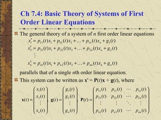
The general theory of a system of n first order linear equations
parallels that of a single nth order linear equation.
This system can be written as x' = P(t)x + g(t), where
)()()()(
)()()()(
)()()()(
2211
222221212
112121111
tgxtpxtpxtpx
tgxtpxtpxtpx
tgxtpxtpxtpx
nnnnnnn
nn
nn
++++=′
++++=′
++++=′
=
=
=
)()()(
)()()(
)()()(
)(,
)(
)(
)(
)(,
)(
)(
)(
)(
21
22221
11211
2
1
2
1
tptptp
tptptp
tptptp
t
tg
tg
tg
t
tx
tx
tx
t
nnnn
n
n
nn
Pgx
2. Vector Solutions of an ODE System
A vector x = φ(t) is a solution of x' = P(t)x + g(t) if the
components of x,
satisfy the system of equations on I: α < t < β.
For comparison, recall that x' = P(t)x + g(t) represents our
system of equations
Assuming P and g continuous on I, such a solution exists by
Theorem 7.1.2.
),(,),(),( 2211 txtxtx nn φφφ ===
)()()()(
)()()()(
)()()()(
2211
222221212
112121111
tgxtpxtpxtpx
tgxtpxtpxtpx
tgxtpxtpxtpx
nnnnnnn
nn
nn
++++=′
++++=′
++++=′
3. Example 1
Consider the homogeneous equation x' = P(t)x below, with
the solutions x as indicated.
To see that x is a solution, substitute x into the equation and
perform the indicated operations:
t
t
t
e
e
e
t 3
3
3
2
1
2
)(;
14
11
=
=
=′ xxx
xx ′=
=
=
=
t
t
t
t
t
t
e
e
e
e
e
e
3
3
3
3
3
3
2
3
6
3
214
11
14
11
4. Homogeneous Case; Vector Function Notation
As in Chapters 3 and 4, we first examine the general
homogeneous equation x' = P(t)x.
Also, the following notation for the vector functions
x(1)
, x(2)
,…, x(k)
,… will be used:
,
)(
)(
)(
)(,,
)(
)(
)(
)(,
)(
)(
)(
)( 2
1
)(
2
22
12
)2(
1
21
11
)1(
=
=
=
tx
tx
tx
t
tx
tx
tx
t
tx
tx
tx
t
nn
n
n
k
nn
xxx
5. Theorem 7.4.1
If the vector functions x(1)
and x(2)
are solutions of the system
x' = P(t)x, then the linear combination c1x(1)
+ c2x(2)
is also a
solution for any constants c1 and c2.
Note: By repeatedly applying the result of this theorem, it
can be seen that every finite linear combination
of solutions x(1)
, x(2)
,…, x(k)
is itself a solution to x' = P(t)x.
)()()( )()2(
2
)1(
1 tctctc k
k xxxx +++=
6. Example 2
Consider the homogeneous equation x' = P(t)x below, with
the two solutions x(1)
and x(2)
as indicated.
Then x = c1x(1)
+ c2x(2)
is also a solution:
−
=
=
=′ −
−
t
t
t
t
e
e
t
e
e
t
2
)(,
2
)(;
14
11 )2(
3
3
)1(
xxxx
x
x
′=
−
+
=
−
+
=
−
+
=
−
−
−
−
−
−
t
t
t
t
t
t
t
t
t
t
t
t
e
e
c
e
e
c
ec
ec
ec
ec
ec
ec
ec
ec
26
3
26
3
214
11
214
11
14
11
23
3
1
2
2
3
1
3
1
2
2
3
1
3
1
7. Theorem 7.4.2
If x(1)
, x(2)
,…, x(n)
are linearly independent solutions of the
system x' = P(t)x for each point in I: α < t < β, then each
solution x = φ(t) can be expressed uniquely in the form
If solutions x(1)
,…, x(n)
are linearly independent for each point
in I: α < t < β, then they are fundamental solutions on I,
and the general solution is given by
)()()( )()2(
2
)1(
1 tctctc n
nxxxx +++=
)()()( )()2(
2
)1(
1 tctctc n
nxxxx +++=
8. The Wronskian and Linear Independence
The proof of Thm 7.4.2 uses the fact that if x(1)
, x(2)
,…, x(n)
are
linearly independent on I, then detX(t) ≠ 0 on I, where
The Wronskian of x(1)
,…, x(n)
is defined as
W[x(1)
,…, x(n)
](t) = detX(t).
It follows that W[x(1)
,…, x(n)
](t) ≠ 0 on I iff x(1)
,…, x(n)
are
linearly independent for each point in I.
,
)()(
)()(
)(
1
111
=
txtx
txtx
t
nnn
n
X
9. Theorem 7.4.3
If x(1)
, x(2)
,…, x(n)
are solutions of the system x' = P(t)x on I: α
< t < β, then the Wronskian W[x(1)
,…, x(n)
](t) is either
identically zero on I or else is never zero on I.
This result enables us to determine whether a given set of
solutions x(1)
, x(2)
,…, x(n)
are fundamental solutions by
evaluating W[x(1)
,…, x(n)
](t) at any point t in α < t < β.
10. Theorem 7.4.4
Let
Let x(1)
, x(2)
,…, x(n)
be solutions of the system x' = P(t)x,
α < t < β, that satisfy the initial conditions
respectively, where t0 is any point in α < t < β. Then
x(1)
, x(2)
,…, x(n)
are fundamental solutions of x' = P(t)x.
=
=
=
1
0
0
0
,,
0
0
1
0
,
0
0
0
1
)()2()1(
n
eee
,)(,,)( )(
0
)()1(
0
)1( nn
tt exex ==