Torque Arm FEA Analysis and Optimization
•
0 likes•1,719 views

Designed a torque arm, with Multi Point Constraints applied to the center of the arm. The FEA software used for this purpose was ABAQUS. The analysis was performed two major element types: Triangular Elements and Quadrilateral Elements, with relatively equal number of nodes in each case and a convergence study was conducted. The aim of the project was to obtain the optimal design parameters of the torque arm by optimization (minimize weight).

Recommended
More Related Content
What's hot
What's hot (20)
Similar to Torque Arm FEA Analysis and Optimization
Similar to Torque Arm FEA Analysis and Optimization (20)
Recently uploaded
Recently uploaded (20)
Torque Arm FEA Analysis and Optimization
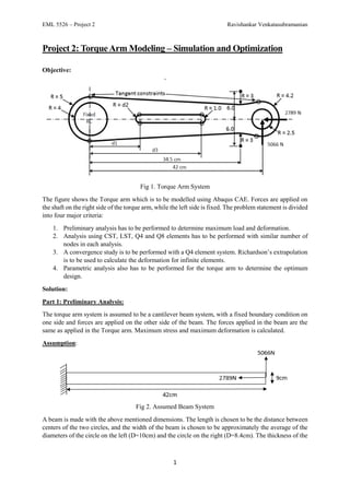
- 1. EML 5526 – Project 2 Ravishankar Venkatasubramanian 1 Project 2: TorqueArm Modeling – Simulation and Optimization Objective: Fig 1. Torque Arm System The figure shows the Torque arm which is to be modelled using Abaqus CAE. Forces are applied on the shaft on the right side of the torque arm, while the left side is fixed. The problem statement is divided into four major criteria: 1. Preliminary analysis has to be performed to determine maximum load and deformation. 2. Analysis using CST, LST, Q4 and Q8 elements has to be performed with similar number of nodes in each analysis. 3. A convergence study is to be performed with a Q4 element system. Richardson’s extrapolation is to be used to calculate the deformation for infinite elements. 4. Parametric analysis also has to be performed for the torque arm to determine the optimum design. Solution: Part 1: Preliminary Analysis: The torque arm system is assumed to be a cantilever beam system, with a fixed boundary condition on one side and forces are applied on the other side of the beam. The forces applied in the beam are the same as applied in the Torque arm. Maximum stress and maximum deformation is calculated. Assumption: Fig 2. Assumed Beam System A beam is made with the above mentioned dimensions. The length is chosen to be the distance between centers of the two circles, and the width of the beam is chosen to be approximately the average of the diameters of the circle on the left (D=10cm) and the circle on the right (D=8.4cm). The thickness of the
- 2. EML 5526 – Project 2 Ravishankar Venkatasubramanian 2 beam is maintained at 1mm. The equations used to calculate the maximum deformation and the maximum stress are directly obtained from mechanics of materials. The problem can be divided into two parts, one is the stress caused due to axial force, and the other is the stress caused due to bending moment. The stress caused due to axial force can be represented by: 𝜎 𝑎𝑥𝑖𝑎𝑙 = 𝐹 𝐴 Where F is the Force applied in the axial direction, and A is the Cross Sectional Area. F=-2789N, A= (1x9 cm2 = 9cm2 ). Placing the values back in the equation, we get: 𝜎 𝑎𝑥𝑖𝑎𝑙 = −2789 9 𝑁/𝑐𝑚2 = −309.88 N/𝑐𝑚2 The stress due to bending is calculated next. It is given by the equation, 𝜎 𝑏𝑒𝑛𝑑𝑖𝑛𝑔 = − 𝑀𝑦 𝐼 Here, M = F*(x), and the value of F=5066N, x=42cm, and therefore, M= (5066x42) = 212772 N/cm2 . The value of y=4.5cm (distance from neutral axis). The moment of inertia is given by: 𝐼 = 𝑏𝑑3 12 = 1 × 93 12 = 60.75 𝑐𝑚4 Substituting the values back into the equation, we get: 𝜎 𝑏𝑒𝑛𝑑𝑖𝑛𝑔 = − 2122772 × 4.5 60.75 = −157242.3704 𝑁/𝑐𝑚2 Therefore, the maximum stress is obtained by the addition of both the values of stresses, i.e., the axial stress and the bending stress. The resultant stress is obtained as: 𝜎 𝑚𝑎𝑥 = 157.552 𝑀𝑃𝑎 The stress calculated from this assumption cannot be directly taken as a reference for the calculations. The actual stress will be higher as there will be the effect of stress concentration around the holes and slots in the original torque arm system. A safe stress concentration factor can be assumed between 1.5 and 2. Taking 1.5 as the stress concentration factor, the maximum stress obtained: 𝜎 𝑚𝑎𝑥−𝑓𝑖𝑛𝑎𝑙 = 157.552 × 1.5 = 236.32 𝑀𝑃𝑎 The value of maximum deformation can be calculated from beam theory: 𝛿 𝑚𝑎𝑥 = 𝑃𝐿3 3𝐸𝐼 The load applied in this case is considered as the bending load only, as the axial load does not contribute to the net deformation. The value of P=5066 N, L=42cm, E=206.8 GPa, I= 60.75 cm4 (as calculated from previous case). The maximum deflection, hence is: 𝛿 𝑚𝑎𝑥 = 5066 × 423 3 × (206.8 × 105) × (60.75) = 0.09958 𝑐𝑚 ~0.1𝑐𝑚
- 3. EML 5526 – Project 2 Ravishankar Venkatasubramanian 3 Since the beam considered is one without any holes or discontinuities, it will be stiff, and hence, the deformation will be low. Therefore, the actual deformation of the torque arm system will be higher than 0.1cm. Part 2: Analysis using CST, LST, Q4 and Q8 element type: The analysis of the torque arm design has to be performed on Abaqus CAE. The design of the system has to be made initially, which is done in a manner that updating the dimensions to other values automatically updates the geometry in a parametric fashion. The dimensions given in the figure are only used, no other extra dimensions are used, and no dimensions have been skipped. Fig 3: Dimensioning of the sketch – Fully Defined Geometry The lines change from yellow to green when a geometry is fully defined, as shown in Fig. 3. Once the drawing part has been completed, a section is formed. A specific thickness (1cm in this case) has to be assigned to the section. The properties of the material are also added to the material section. Boundary conditions are applied to the center of the circles in both cases, which cannot be directly applied. To apply the boundary conditions and loads on the system, the concept of slave nodes is used. Slave nodes are points on the periphery of the circle, which are connected to the load application point through rigid beam elements. These help in transferring the loads from the load application point to the periphery/section. The meshing is initially performed for a CST element, for a fine mesh. The mesh was made structured to obtain a good shape of the elements, providing a good mesh. The finest mesh had a mesh ratio of 0.59, which provided the number of nodes equal to 968. The meshing was then performed for a Q4 element, trying the keep the number of nodes constant. The number of nodes in Q4 was found to be 968 for the lowest mesh ratio possible. The meshing was then performed for an LST element, keeping the lowest mesh ratio possible, while keeping the number of nodes below 1000. The number of nodes in LST was found to be 998. The final meshing performed was for the Q8 element, where the number of nodes was found to be 979. Therefore, the number of nodes used in all the elements were fairly constant, and hence a comparison can be made for the stress and deformation values for all the elements, which is tabulated in Table 1. The meshing and stress output of a CST element is shown in Fig. 3.
- 4. EML 5526 – Project 2 Ravishankar Venkatasubramanian 4 Fig 3. CST Element - Stress Table 1: Stress and Deformation comparison The stress and deformation was calculated at the finest mesh provides a good comparison of stress and deformation for all the element types. The CST element is stiff to bending, and hence, its deformation and also the stress is low. The Q4 element on the other hand, is not as stiff to bending as the CST element is, but it still is stiff to bending. The LST element can represent bending almost perfectly, as it has the complete polynomial in its deflection equation. But, since the geometry is not just plain bending, and it has stress concentration due to the existence of circular holes in its geometry, LST element only makes an attempt at reaching the accurate solution. The Q8 element on the other hand, has the second order polynomial in its deflection equation, and it is much more accurate than the LST element in its calculation of stress and deformation. Part 3: Convergence Study: The convergence study provides an estimate on the mesh size to be used while making calculations using FEA. The concept of the study is pretty straightforward. When the deformation value of the system reaches a saturation/converges, it means that further refinement of the mesh (decrease mesh size) will not improve the result by a considerable amount. In this case, the analysis was performed only for a Q4 element. Since the student edition of Abaqus CAE restricts the total number of nodes by 1000, the maximum number of nodes used in this study was 968. The corresponding number of elements is 810. The meshing was started from 140 elements, for a coarse element system and then it progressed to 364 elements for a medium mesh and then went on to 810 elements for the finest mesh. The mesh size was constantly reduced from 1.7 to 0.59. The reasonable mesh size is 0.59. The corresponding stress and deformation was calculated at each of these changes, as represented in Table 2. Element Type Nodes Elements Stress (MPa) Deformation (cm) Deformation at shaft (cm) CST 968 1620 157 0.1374 0.119279 Q4 968 810 188.3 0.1404 0.122179 LST 998 422 198.7 0.1407 0.122418 Q8 978 269 215.5 0.1415 0.123192
- 5. EML 5526 – Project 2 Ravishankar Venkatasubramanian 5 Table 2: Convergence Study of Q4 Element The convergence study provides us with data which shows that the maximum deformation at the center of the shaft at 968 nodes and 810 elements is 0.122179, which is the highest amount as calculated by a Q4 element. The graph in Fig. 5 shows the same trend in deformation at the center of the shaft. Fig 5: Convergence study – Deformation vs Number of Elements Richardson’s Extrapolation: The number of elements used in FEA analysis is finite. But accurate data can be obtained if the number of elements is infinite. Hence, the formula of Richardson’s extrapolation is used to determine the deformation at infinite Q4 elements. The equation of Richardson’s extrapolation is given by: ∅∞ = ∅1ℎ2 𝑞 − ∅2ℎ1 𝑞 ℎ2 𝑞 − ℎ1 𝑞 In this case, ∅ is the deformation at the center of the shaft, while h is the mesh size. For this analysis, we use the finest mesh and the next finest mesh as a reference to calculate the deformation at infinite Nodes Elements Stress (MPa) Maximum Deformation (cm) Deformation at Center Shaft (cm) Mesh Size (h) 199 140 167.6 0.1362 0.118089 1.7 213 150 169.2 0.1366 0.118465 1.5 291 214 171.5 0.138 0.119847 1.3 365 278 175.4 0.1385 0.120265 1.1 468 364 176.1 0.1392 0.120958 0.9 667 536 183.5 0.1403 0.121575 0.7 968 810 188.3 0.1404 0.122179 0.59 0.1175 0.118 0.1185 0.119 0.1195 0.12 0.1205 0.121 0.1215 0.122 0.1225 0 100 200 300 400 500 600 700 800 900 Deformation(cm) Number of Elements Deformation at the center of the shaft
- 6. EML 5526 – Project 2 Ravishankar Venkatasubramanian 6 elements. Substitute ∅1= 0.121575, ∅2= 0.122179 and h1=0.7 and h2=0.59. Since Q4 has a first order complete polynomial, we know that p=1. Hence, the value of q = p+1= 2. Therefore, take q = 2. ∅∞ = 0.121575 × 0.592 − 0.122179 × 0.72 0.592 − 0.72 => ∅∞ = 0.123660694 𝑐𝑚 It can be noticed that the deformation calculated at infinity is larger than the deformation calculated at 968 nodes. Part 4: Parametric Study: The parametric study is performed in order to obtain the optimum design, with lowest mass. The formula mentioned in the question provides a method to optimise the design with lowest material use and also able to withstand a stress of 240 MPa. This analysis is done by varying the values of d1, d2 and d3 from Fig 1 with respect to the equations mentioned below: d1= 10d + 8 d2 = -2d + 3 d3 = -9d + 36 where d varies from [0,1]. This variation is made into ten increments, starting from d=0, in steps of 0.1. The parametric study is performed, changing the design, while maintaining the mesh size. Although Q8 provides more accurate results in the parametric study, Q4 is used in this study because of the restriction of maintaining the mesh size as the one used in the convergence study. The study is performed to determine the maximum deformation at the edge and maximum stress values. With the change in value of d, there is a change in the stress and deformation of the design. The change in dimensions for every step increase of change in d is mentioned in Table 3. Table 3: Change in dimensions These change in dimensions are applied to the geometry. An example of the changed geometry is given in Fig 6. d d1 d2 d3 0 8 3 36 0.1 9 2.8 35.1 0.2 10 2.6 34.2 0.3 11 2.4 33.3 0.4 12 2.2 32.4 0.5 13 2 31.5 0.6 14 1.8 30.6 0.7 15 1.6 29.7 0.8 16 1.4 28.8 0.9 17 1.2 27.9 1 18 1 27
- 7. EML 5526 – Project 2 Ravishankar Venkatasubramanian 7 Fig. 6: Example of dimensionally altered sketch. The change in dimensions provides a changed value of stress and deformation. For the purpose of parametric analysis, mass has also been calculated. The optimum design must be able to withstand a maximum load of 240 MPa and it must also have the lowest mass. For this analysis, the formula used is given as: Where α=100 (penalty number). This formula is used to calculate the value of f(d), data is presented in Table 4. Parameter Initial Mass Mass Stress Max Displacement max f(d) d=0 2.31 1.5649 475.1 0.3483 98.63577922 d=0.1 2.31 1.68001 430.7 0.2867 80.18561039 d=0.2 2.31 1.78836 397.8 0.2445 66.52418182 d=0.3 2.31 1.88973 358.2 0.2125 50.06806494 d=0.4 2.31 1.98409 317.4 0.1888 33.10891342 d=0.5 2.31 2.07148 282.2 0.1708 18.48007792 d=0.6 2.31 2.15187 244.8 0.1577 2.931545455 d=0.7 2.31 2.22526 211.7 0.1477 0.963316017 d=0.8 2.31 2.29169 191.7 0.1408 0.992073593 d=0.9 2.31 2.35109 175.1 0.1357 1.017787879 d=1 2.31 2.40348 160.7 0.1321 1.040467532 Table 4: Parametric Analysis It can be noticed from the table that the value of f(d) reduces from a high value to a low value and then increases again. A graphical representation of f(d) vs d is shown in Fig 7.
- 8. EML 5526 – Project 2 Ravishankar Venkatasubramanian 8 Fig 7: Plot of f(d) vs d The plot of f(d) vs d shows that the value of dopt might exist between d=0.7 and d=0.8. From the graph, it can be told that the minimum is at d=0.79. Hence, we take dopt=0.79. Therefore, the dimensions vary: d1= 10d + 8 = 15.9 d2 = -2d + 3 = 1.42 d3 = -9d + 36 = 28.89. Substituting these dimensions back into the drawing, we obtain the value of stress, deformation and mass. They are represented in Fig 8 and Fig 9. Fig 8: Stress obtained in Optimum design case -20 0 20 40 60 80 100 120 0 0.2 0.4 0.6 0.8 1 1.2 f(d) Value of d f(d) vs Parameter d
- 9. EML 5526 – Project 2 Ravishankar Venkatasubramanian 9 Fig. 9: Displacement obtained in Optimum design case Therefore, the optimum mass, maximum stress and maximum displacement are determined by running analysis and finding out the design and the parameters of the optimum design are represented in Table 5. Table 5: Optimum Design The optimum design condition has been obtained and the problem has been solved. Parameter d=0.79 d1 15.9 d2 1.42 d3 28.89 Initial Mass 2.31 Mass 2.28683 Stress Max 192.5 Displacement max 0.1413