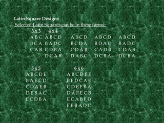
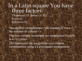
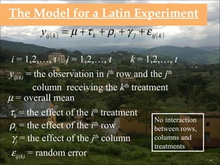
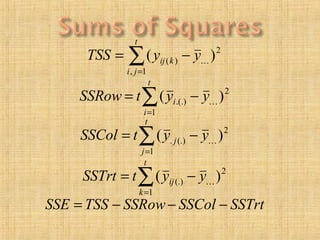
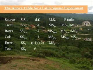
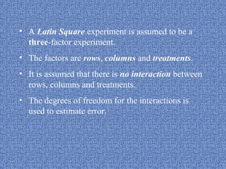
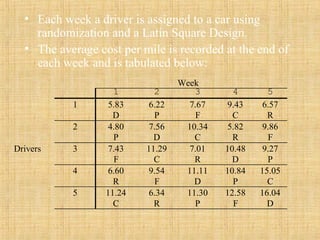
This document discusses Latin square designs, which are experimental designs used to study the effects of multiple factors. A Latin square design has the same number of treatments, rows, and columns, with each treatment occurring once in each row and column. This allows researchers to study the effects of treatments, rows, and columns while controlling for interactions between them. The document provides examples of 3x3 and 4x4 Latin squares and explains how to analyze the results using ANOVA.

3. Latin Square Designs
Selected Latin Squares can be in these forms::
3 x 3 4 x 4
A B C A B C D A B C D A B C D A B C D
B C A B A D C B C D A B D A C B A D C
C A B C D B A C D A B C A D B C D A B
D C A B D A B C D C B A D C B A
5 x 5 6 x 6
A B C D E A B C D E F
B A E C D B F D C A E
C D A E B C D E F B A
D E B A C D A F E C B
E C D B A E C A B F D
F E B A D C

4.  A Latin square is a square array of objects
(letters A, B, C, …) such that each object
appears once and only once in each row and
each column. Example - 4 x 4 Latin Square.
A B C D
B C D A
C D A B
D A B C

5.  We have seen that in random block
design ,the whole experiment area
is divided into the homogenous
block and randomisation kept
restricted within the block .but in
latin square design the exp. Rows
and columns are equal and each
treatment occurs only once in a row
and column.

6. In a Latin square You have
three factors:
 Treatments (t) (letters A, B, C, …)
 Rows (t)
 Columns (t)
The number of treatments = the number of rows =
the number of colums = t.
The row-column treatments are represented by cells
in a t x t array.
The treatments are assigned to row-column
combinations using a Latin-square arrangement

7. The Model for a Latin Experiment
( ) ( )kijjikkijy εγρτµ ++++=
i = 1,2,…, t j = 1,2,…, t
yij(k) = the observation in ith
row and the jth
column receiving the kth
treatment
µ = overall mean
τk = the effect of the ith
treatment
ρi = the effect of the ith
row
εij(k) = random error
k = 1,2,…, t
γj = the effect of the jth
column
No interaction
between rows,
columns and
treatments

8. SSTrtSSColSSRowTSSSSE
yytSSTrt
yytSSCol
yytSSRow
yyTSS
t
k
ij
t
j
j
t
i
i
t
ji
kij
−−−=
−=
−=
−=
−=
∑
∑
∑
∑
=
=
=
=
1
2
(.)
1
2
(.).
1
2
.(.)
1,
2
)(
)(
)(
)(
)(





9. The Anova Table for a Latin Square Experiment
Source S.S. d.f. M.S. F ratio
Treat SSTr t-1 MSTr MSTr /MSE
Rows SSRow t-1 MSRow MSRow /MSE
Cols SSCol t-1 MSCol MSCol /MSE
Error SSE (t-1)(t-2) MSE
Total SST t2
- 1

10. • A Latin Square experiment is assumed to be a
three-factor experiment.
• The factors are rows, columns and treatments.
• It is assumed that there is no interaction between
rows, columns and treatments.
• The degrees of freedom for the interactions is
used to estimate error.

11. A courier company is interested in deciding
between five brands (D,P,F,C and R) of car for
its next purchase of fleet cars.
• The brands are all comparable in purchase price.
• The company wants to carry out a study that will
enable them to compare the brands with respect to
operating costs.
• For this purpose they select five drivers (Rows).
• In addition the study will be carried out over a
five week period (Columns = weeks).

12. • Each week a driver is assigned to a car using
randomization and a Latin Square Design.
• The average cost per mile is recorded at the end of
each week and is tabulated below:
Week
1 2 3 4 5
1 5.83 6.22 7.67 9.43 6.57
D P F C R
2 4.80 7.56 10.34 5.82 9.86
P D C R F
Drivers 3 7.43 11.29 7.01 10.48 9.27
F C R D P
4 6.60 9.54 11.11 10.84 15.05
R F D P C
5 11.24 6.34 11.30 12.58 16.04
C R P F D

13. The Anova Table for Example
Source S.S. d.f. M.S. F ratio
Week 51.17887 4 12.79472 16.06
Driver 69.44663 4 17.36166 21.79
Car 70.90402 4 17.72601 22.24
Error 9.56315 12 0.79693
Total 201.09267 24

14.  Advantage:
 Allows the experimenter to control two sources of
variation
 Disadvantages:
 The experiment becomes very large if the number of
treatments is large
 The statistical analysis is complicated by missing
plots and misassigned treatments
 Error df is small if there are only a few treatments
 This limitation can be overcome by repeating a small
Latin Square and then combining the experiments -
 a 3x3 Latin Square repeated 4 times
 a 4x4 Latin Square repeated 2 times