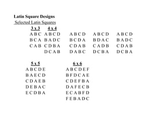
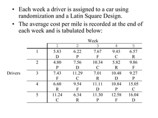
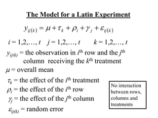
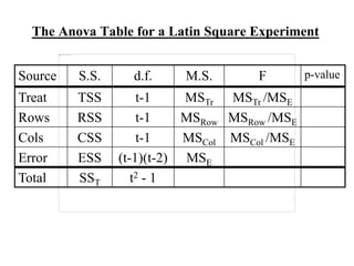
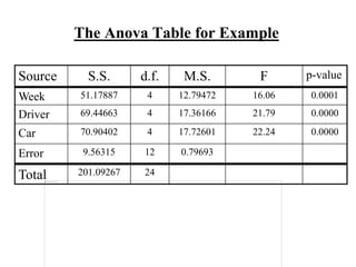
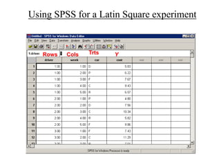
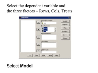
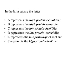
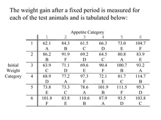
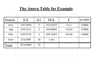
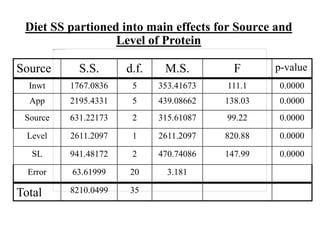
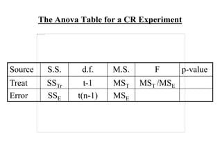
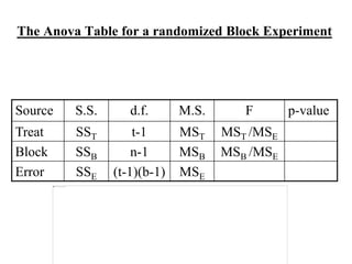
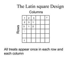
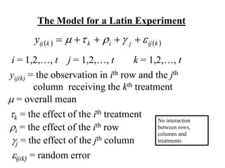
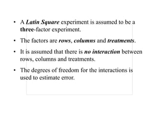
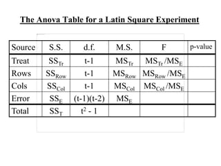
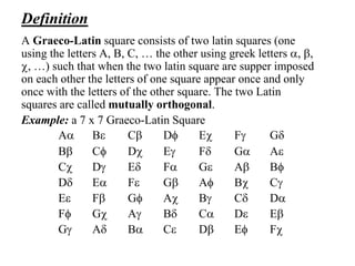
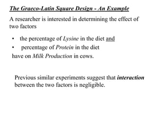
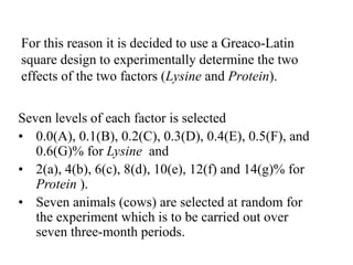
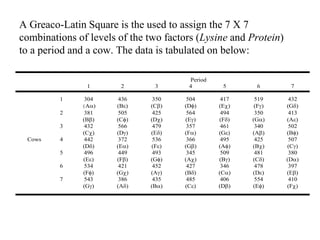
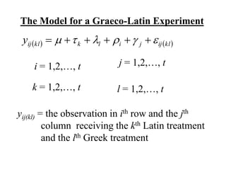
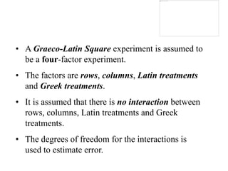
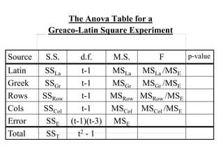
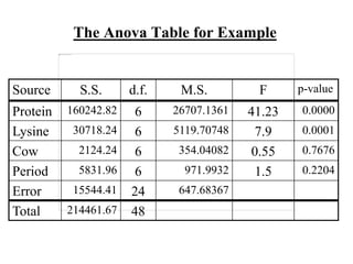
Presentation
• Name: Nadeem Altaf
• Roll #: BSTF17E-122®
• Topic: Graeco Latin Square Design
• Present To: Mam Noureen Akhter
Latin Square Designs
Selected Latin Squares
3 x 3 4 x 4
A B C A B C D A B C D A B C D A B C D
B C A B A D C B C D A B D A C B A D C
C A B C D B A C D A B C A D B C D A B
D C A B D A B C D C B A D C B A
5 x 5 6 x 6
A B C D E A B C D E F
B A E C D B F D C A E
C D A E B C D E F B A
D E B A C D A F E C B
E C D B A E C A B F D
F E B A D C
A Latin Square
Definition
• A Latin square is a square array of objects (letters A,
B, C, …) such that each object appears once and only
once in each row and each column. Example - 4 x 4
Latin Square.
A B C D
B C D A
C D A B
D A B C
In a Latin square You have three factors:
• Treatments (t) (letters A, B, C, …)
• Rows (t)
• Columns (t)
The number of treatments = the number of rows =
the number of colums = t.
The row-column treatments are represented by cells
in a t x t array.
The treatments are assigned to row-column
combinations using a Latin-square arrangement
Example
A courier company is interested in deciding
between five brands (D,P,F,C and R) of car
for its next purchase of fleet cars.
• The brands are all comparable in purchase price.
• The company wants to carry out a study that will
enable them to compare the brands with respect to
operating costs.
• For this purpose they select five drivers (Rows).
• In addition the study will be carried out over a
five week period (Columns = weeks).
• Each week a driver is assigned to a car using
randomization and a Latin Square Design.
• The average cost per mile is recorded at the end of
each week and is tabulated below:
Week
1 2 3 4 5
1 5.83 6.22 7.67 9.43 6.57
D P F C R
2 4.80 7.56 10.34 5.82 9.86
P D C R F
Drivers 3 7.43 11.29 7.01 10.48 9.27
F C R D P
4 6.60 9.54 11.11 10.84 15.05
R F D P C
5 11.24 6.34 11.30 12.58 16.04
C R P F D
The Model for a Latin Experiment
   
k
ij
j
i
k
k
ij
y 



 




i = 1,2,…, t j = 1,2,…, t
yij(k) = the observation in ith row and the jth
column receiving the kth treatment
 = overall mean
k = the effect of the ith treatment
i = the effect of the ith row
ij(k) = random error
k = 1,2,…, t
j = the effect of the jth column
No interaction
between rows,
columns and
treatments
• A Latin Square experiment is assumed to be a
three-factor experiment.
• The factors are rows, columns and treatments.
• It is assumed that there is no interaction between
rows, columns and treatments.
• The degrees of freedom for the interactions is
used to estimate error.
The Anova Table for a Latin Square Experiment
Source S.S. d.f. M.S. F p-value
Treat TSS t-1 MSTr MSTr /MSE
Rows RSS t-1 MSRow MSRow /MSE
Cols CSS t-1 MSCol MSCol /MSE
Error ESS (t-1)(t-2) MSE
Total SST t2 - 1
The Anova Table for Example
Source S.S. d.f. M.S. F p-value
Week 51.17887 4 12.79472 16.06 0.0001
Driver 69.44663 4 17.36166 21.79 0.0000
Car 70.90402 4 17.72601 22.24 0.0000
Error 9.56315 12 0.79693
Total 201.09267 24
Using SPSS for a Latin Square experiment
Rows Cols Trts Y
Select
Analyze->General Linear Model->Univariate
Select the dependent variable and
the three factors – Rows, Cols, Treats
Select Model
Identify a model that has only main
effects for Rows, Cols, Treats
Tests of Between-Subjects Effects
Dependent Variable: COST
191.530a
12 15.961 20.028 .000
2120.050 1 2120.050 2660.273 .000
69.447 4 17.362 21.786 .000
51.179 4 12.795 16.055 .000
70.904 4 17.726 22.243 .000
9.563 12 .797
2321.143 25
201.093 24
Source
Corrected Model
Intercept
DRIVER
WEEK
CAR
Error
Total
Corrected Total
Type III
Sum of
Squares df
Mean
Square F Sig.
R Squared = .952 (Adjusted R Squared = .905)
a.
The ANOVA table produced by SPSS
Example 2
In this Experiment we are again interested in how
weight gain (Y) in rats is affected by Source of
protein (Beef, Cereal, and Pork) and by Level of
Protein (High or Low).
There are a total of t = 3 X 2 = 6 treatment
combinations of the two factors.
• Beef -High Protein
• Cereal-High Protein
• Pork-High Protein
• Beef -Low Protein
• Cereal-Low Protein and
• Pork-Low Protein
In this example we will consider using a Latin Square
design
Six Initial Weight categories are identified for the
test animals in addition to Six Appetite categories.
• A test animal is then selected from each of the 6 X
6 = 36 combinations of Initial Weight and
Appetite categories.
• A Latin square is then used to assign the 6 diets to
the 36 test animals in the study.
In the latin square the letter
• A represents the high protein-cereal diet
• B represents the high protein-pork diet
• C represents the low protein-beef Diet
• D represents the low protein-cereal diet
• E represents the low protein-pork diet and
• F represents the high protein-beef diet.
The weight gain after a fixed period is measured for
each of the test animals and is tabulated below:
Appetite Category
1 2 3 4 5 6
1 62.1 84.3 61.5 66.3 73.0 104.7
A B C D E F
2 86.2 91.9 69.2 64.5 80.8 83.9
B F D C A E
Initial 3 63.9 71.1 69.6 90.4 100.7 93.2
Weight C D E F B A
Category 4 68.9 77.2 97.3 72.1 81.7 114.7
D A F E C B
5 73.8 73.3 78.6 101.9 111.5 95.3
E C A B F D
6 101.8 83.8 110.6 87.9 93.5 103.8
F E B A D C
The Anova Table for Example
Source S.S. d.f. M.S. F p-value
Inwt 1767.0836 5 353.41673 111.1 0.0000
App 2195.4331 5 439.08662 138.03 0.0000
Diet 4183.9132 5 836.78263 263.06 0.0000
Error 63.61999 20 3.181
Total 8210.0499 35
Diet SS partioned into main effects for Source and
Level of Protein
Source S.S. d.f. M.S. F p-value
Inwt 1767.0836 5 353.41673 111.1 0.0000
App 2195.4331 5 439.08662 138.03 0.0000
Source 631.22173 2 315.61087 99.22 0.0000
Level 2611.2097 1 2611.2097 820.88 0.0000
SL 941.48172 2 470.74086 147.99 0.0000
Error 63.61999 20 3.181
Total 8210.0499 35
Experimental Design
Of interest: to compare t treatments
(the treatment combinations of one or
several factors)
The Completely Randomized Design
Treats
1 2 3 … t
Experimental units randomly assigned to
treatments
The Model for a CR Experiment
ij
i
ij
y 

 


i = 1,2,…, t j = 1,2,…, n
yij = the observation in jth observation
receiving the ith treatment
 = overall mean
i = the effect of the ith
treatment
ij = random error
The Anova Table for a CR Experiment
Source S.S. d.f. M.S. F p-value
Treat SSTr t-1 MST MST /MSE
Error SSE t(n-1) MSE
Randomized Block Design
Blocks
All treats appear once in each block
1
2
3
⁞
t
1
2
3
⁞
t
1
2
3
⁞
t
1
2
3
⁞
t
1
2
3
⁞
t
1
2
3
⁞
t
1
2
3
⁞
t
1
2
3
⁞
t
1
2
3
⁞
t
The Model for a RB Experiment
ij
j
i
ij
y 


 



i = 1,2,…, t j = 1,2,…, b
yij = the observation in jth block receiving the ith
treatment
 = overall mean
i = the effect of the ith treatment
ij = random error
j = the effect of the jth block
No interaction
between blocks
and treatments
• A Randomized Block experiment is
assumed to be a two-factor experiment.
• The factors are blocks and treatments.
• It is assumed that there is no interaction
between blocks and treatments.
• The degrees of freedom for the interaction is
used to estimate error.
The Anova Table for a randomized Block Experiment
Source S.S. d.f. M.S. F p-value
Treat SST t-1 MST MST /MSE
Block SSB n-1 MSB MSB /MSE
Error SSE (t-1)(b-1) MSE
The Latin square Design
All treats appear once in each row and
each column
Columns
Rows 1
2
3
⁞
t
2
3
t
1
1
3
2
The Model for a Latin Experiment
   
k
ij
j
i
k
k
ij
y 



 




i = 1,2,…, t j = 1,2,…, t
yij(k) = the observation in ith row and the jth
column receiving the kth treatment
 = overall mean
k = the effect of the ith treatment
i = the effect of the ith row
ij(k) = random error
k = 1,2,…, t
j = the effect of the jth column
No interaction
between rows,
columns and
treatments
• A Latin Square experiment is assumed to be a
three-factor experiment.
• The factors are rows, columns and treatments.
• It is assumed that there is no interaction between
rows, columns and treatments.
• The degrees of freedom for the interactions is
used to estimate error.
The Anova Table for a Latin Square Experiment
Source S.S. d.f. M.S. F p-value
Treat SSTr t-1 MSTr MSTr /MSE
Rows SSRow t-1 MSRow MSRow /MSE
Cols SSCol t-1 MSCol MSCol /MSE
Error SSE (t-1)(t-2) MSE
Total SST t2 - 1
Graeco-Latin Square Design
Mutually orthogonal Squares
Definition
A Graeco-Latin square consists of two latin squares (one
using the letters A, B, C, … the other using greek letters a, ,
c, …) such that when the two latin square are supper imposed
on each other the letters of one square appear once and only
once with the letters of the other square. The two Latin
squares are called mutually orthogonal.
Example: a 7 x 7 Graeco-Latin Square
Aa B C Df Ec F Gd
B Cf Dc E Fd Ga A
Cc D Ed Fa G A Bf
Dd Ea F G Af Bc C
E F Gf Ac B Cd Da
Ff Gc A Bd Ca D E
G Ad Ba C D Ef Fc
Note:
There exists at most (t –1) t x t Latin squares L1, L2,
…, Lt-1 such that any pair are mutually orthogonal.
e.g. It is possible that there exists a set of six 7 x 7
mutually orthogonal Latin squares L1, L2, L3, L4, L5,
L6 .
The Graeco-Latin Square Design - An Example
A researcher is interested in determining the effect of
two factors
• the percentage of Lysine in the diet and
• percentage of Protein in the diet
have on Milk Production in cows.
Previous similar experiments suggest that interaction
between the two factors is negligible.
For this reason it is decided to use a Greaco-Latin
square design to experimentally determine the two
effects of the two factors (Lysine and Protein).
Seven levels of each factor is selected
• 0.0(A), 0.1(B), 0.2(C), 0.3(D), 0.4(E), 0.5(F), and
0.6(G)% for Lysine and
• 2(a), 4(b), 6(c), 8(d), 10(e), 12(f) and 14(g)% for
Protein ).
• Seven animals (cows) are selected at random for
the experiment which is to be carried out over
seven three-month periods.
A Greaco-Latin Square is the used to assign the 7 X 7
combinations of levels of the two factors (Lysine and Protein)
to a period and a cow. The data is tabulated on below:
Period
1 2 3 4 5 6 7
1 304 436 350 504 417 519 432
(Aa (B (C (Df (Ec (F (Gd
2 381 505 425 564 494 350 413
  B (Cf (Dc (E (Fd (Ga (A
3 432 566 479 357 461 340 502
(Cc (D (Ed (Fa (G (A (Bf
Cows 4 442 372 536 366 495 425 507
(Dd (Ea (F (G (Af (Bc (C
5 496 449 493 345 509 481 380
(E (F (Gf (Ac (B (Cd (Da
6 534 421 452 427 346 478 397
(Ff (Gc (A (Bd (Ca (D (E
7 543 386 435 485 406 554 410
(G (Ad (Ba (C (D (Ef (Fc
The Model for a Graeco-Latin Experiment
   
kl
ij
j
i
l
k
kl
ij
y 




 





i = 1,2,…, t j = 1,2,…, t
yij(kl) = the observation in ith row and the jth
column receiving the kth Latin treatment
and the lth Greek treatment
k = 1,2,…, t l = 1,2,…, t
 = overall mean
k = the effect of the kth Latin treatment
i = the effect of the ith row
ij(k) = random error
j = the effect of the jth column
No interaction between rows, columns,
Latin treatments and Greek treatments
l = the effect of the lth Greek treatment
• A Graeco-Latin Square experiment is assumed to
be a four-factor experiment.
• The factors are rows, columns, Latin treatments
and Greek treatments.
• It is assumed that there is no interaction between
rows, columns, Latin treatments and Greek
treatments.
• The degrees of freedom for the interactions is
used to estimate error.
The Anova Table for a
Greaco-Latin Square Experiment
Source S.S. d.f. M.S. F p-value
Latin SSLa t-1 MSLa MSLa /MSE
Greek SSGr t-1 MSGr MSGr /MSE
Rows SSRow t-1 MSRow MSRow /MSE
Cols SSCol t-1 MSCol MSCol /MSE
Error SSE (t-1)(t-3) MSE
Total SST t2 - 1
The Anova Table for Example
Source S.S. d.f. M.S. F p-value
Protein 160242.82 6 26707.1361 41.23 0.0000
Lysine 30718.24 6 5119.70748 7.9 0.0001
Cow 2124.24 6 354.04082 0.55 0.7676
Period 5831.96 6 971.9932 1.5 0.2204
Error 15544.41 24 647.68367
Total 214461.67 48
Next topic: Incomplete Block
designs

Graeco Latin Square Design

  • 1.
    Presentation • Name: NadeemAltaf • Roll #: BSTF17E-122® • Topic: Graeco Latin Square Design • Present To: Mam Noureen Akhter
  • 2.
  • 3.
    Latin Square Designs SelectedLatin Squares 3 x 3 4 x 4 A B C A B C D A B C D A B C D A B C D B C A B A D C B C D A B D A C B A D C C A B C D B A C D A B C A D B C D A B D C A B D A B C D C B A D C B A 5 x 5 6 x 6 A B C D E A B C D E F B A E C D B F D C A E C D A E B C D E F B A D E B A C D A F E C B E C D B A E C A B F D F E B A D C
  • 4.
  • 5.
    Definition • A Latinsquare is a square array of objects (letters A, B, C, …) such that each object appears once and only once in each row and each column. Example - 4 x 4 Latin Square. A B C D B C D A C D A B D A B C
  • 6.
    In a Latinsquare You have three factors: • Treatments (t) (letters A, B, C, …) • Rows (t) • Columns (t) The number of treatments = the number of rows = the number of colums = t. The row-column treatments are represented by cells in a t x t array. The treatments are assigned to row-column combinations using a Latin-square arrangement
  • 7.
    Example A courier companyis interested in deciding between five brands (D,P,F,C and R) of car for its next purchase of fleet cars. • The brands are all comparable in purchase price. • The company wants to carry out a study that will enable them to compare the brands with respect to operating costs. • For this purpose they select five drivers (Rows). • In addition the study will be carried out over a five week period (Columns = weeks).
  • 8.
    • Each weeka driver is assigned to a car using randomization and a Latin Square Design. • The average cost per mile is recorded at the end of each week and is tabulated below: Week 1 2 3 4 5 1 5.83 6.22 7.67 9.43 6.57 D P F C R 2 4.80 7.56 10.34 5.82 9.86 P D C R F Drivers 3 7.43 11.29 7.01 10.48 9.27 F C R D P 4 6.60 9.54 11.11 10.84 15.05 R F D P C 5 11.24 6.34 11.30 12.58 16.04 C R P F D
  • 9.
    The Model fora Latin Experiment     k ij j i k k ij y           i = 1,2,…, t j = 1,2,…, t yij(k) = the observation in ith row and the jth column receiving the kth treatment  = overall mean k = the effect of the ith treatment i = the effect of the ith row ij(k) = random error k = 1,2,…, t j = the effect of the jth column No interaction between rows, columns and treatments
  • 10.
    • A LatinSquare experiment is assumed to be a three-factor experiment. • The factors are rows, columns and treatments. • It is assumed that there is no interaction between rows, columns and treatments. • The degrees of freedom for the interactions is used to estimate error.
  • 11.
    The Anova Tablefor a Latin Square Experiment Source S.S. d.f. M.S. F p-value Treat TSS t-1 MSTr MSTr /MSE Rows RSS t-1 MSRow MSRow /MSE Cols CSS t-1 MSCol MSCol /MSE Error ESS (t-1)(t-2) MSE Total SST t2 - 1
  • 12.
    The Anova Tablefor Example Source S.S. d.f. M.S. F p-value Week 51.17887 4 12.79472 16.06 0.0001 Driver 69.44663 4 17.36166 21.79 0.0000 Car 70.90402 4 17.72601 22.24 0.0000 Error 9.56315 12 0.79693 Total 201.09267 24
  • 13.
    Using SPSS fora Latin Square experiment Rows Cols Trts Y
  • 14.
  • 15.
    Select the dependentvariable and the three factors – Rows, Cols, Treats Select Model
  • 16.
    Identify a modelthat has only main effects for Rows, Cols, Treats
  • 17.
    Tests of Between-SubjectsEffects Dependent Variable: COST 191.530a 12 15.961 20.028 .000 2120.050 1 2120.050 2660.273 .000 69.447 4 17.362 21.786 .000 51.179 4 12.795 16.055 .000 70.904 4 17.726 22.243 .000 9.563 12 .797 2321.143 25 201.093 24 Source Corrected Model Intercept DRIVER WEEK CAR Error Total Corrected Total Type III Sum of Squares df Mean Square F Sig. R Squared = .952 (Adjusted R Squared = .905) a. The ANOVA table produced by SPSS
  • 18.
    Example 2 In thisExperiment we are again interested in how weight gain (Y) in rats is affected by Source of protein (Beef, Cereal, and Pork) and by Level of Protein (High or Low). There are a total of t = 3 X 2 = 6 treatment combinations of the two factors. • Beef -High Protein • Cereal-High Protein • Pork-High Protein • Beef -Low Protein • Cereal-Low Protein and • Pork-Low Protein
  • 19.
    In this examplewe will consider using a Latin Square design Six Initial Weight categories are identified for the test animals in addition to Six Appetite categories. • A test animal is then selected from each of the 6 X 6 = 36 combinations of Initial Weight and Appetite categories. • A Latin square is then used to assign the 6 diets to the 36 test animals in the study.
  • 20.
    In the latinsquare the letter • A represents the high protein-cereal diet • B represents the high protein-pork diet • C represents the low protein-beef Diet • D represents the low protein-cereal diet • E represents the low protein-pork diet and • F represents the high protein-beef diet.
  • 21.
    The weight gainafter a fixed period is measured for each of the test animals and is tabulated below: Appetite Category 1 2 3 4 5 6 1 62.1 84.3 61.5 66.3 73.0 104.7 A B C D E F 2 86.2 91.9 69.2 64.5 80.8 83.9 B F D C A E Initial 3 63.9 71.1 69.6 90.4 100.7 93.2 Weight C D E F B A Category 4 68.9 77.2 97.3 72.1 81.7 114.7 D A F E C B 5 73.8 73.3 78.6 101.9 111.5 95.3 E C A B F D 6 101.8 83.8 110.6 87.9 93.5 103.8 F E B A D C
  • 22.
    The Anova Tablefor Example Source S.S. d.f. M.S. F p-value Inwt 1767.0836 5 353.41673 111.1 0.0000 App 2195.4331 5 439.08662 138.03 0.0000 Diet 4183.9132 5 836.78263 263.06 0.0000 Error 63.61999 20 3.181 Total 8210.0499 35
  • 23.
    Diet SS partionedinto main effects for Source and Level of Protein Source S.S. d.f. M.S. F p-value Inwt 1767.0836 5 353.41673 111.1 0.0000 App 2195.4331 5 439.08662 138.03 0.0000 Source 631.22173 2 315.61087 99.22 0.0000 Level 2611.2097 1 2611.2097 820.88 0.0000 SL 941.48172 2 470.74086 147.99 0.0000 Error 63.61999 20 3.181 Total 8210.0499 35
  • 24.
    Experimental Design Of interest:to compare t treatments (the treatment combinations of one or several factors)
  • 25.
    The Completely RandomizedDesign Treats 1 2 3 … t Experimental units randomly assigned to treatments
  • 26.
    The Model fora CR Experiment ij i ij y       i = 1,2,…, t j = 1,2,…, n yij = the observation in jth observation receiving the ith treatment  = overall mean i = the effect of the ith treatment ij = random error
  • 27.
    The Anova Tablefor a CR Experiment Source S.S. d.f. M.S. F p-value Treat SSTr t-1 MST MST /MSE Error SSE t(n-1) MSE
  • 28.
    Randomized Block Design Blocks Alltreats appear once in each block 1 2 3 ⁞ t 1 2 3 ⁞ t 1 2 3 ⁞ t 1 2 3 ⁞ t 1 2 3 ⁞ t 1 2 3 ⁞ t 1 2 3 ⁞ t 1 2 3 ⁞ t 1 2 3 ⁞ t
  • 29.
    The Model fora RB Experiment ij j i ij y         i = 1,2,…, t j = 1,2,…, b yij = the observation in jth block receiving the ith treatment  = overall mean i = the effect of the ith treatment ij = random error j = the effect of the jth block No interaction between blocks and treatments
  • 30.
    • A RandomizedBlock experiment is assumed to be a two-factor experiment. • The factors are blocks and treatments. • It is assumed that there is no interaction between blocks and treatments. • The degrees of freedom for the interaction is used to estimate error.
  • 31.
    The Anova Tablefor a randomized Block Experiment Source S.S. d.f. M.S. F p-value Treat SST t-1 MST MST /MSE Block SSB n-1 MSB MSB /MSE Error SSE (t-1)(b-1) MSE
  • 32.
    The Latin squareDesign All treats appear once in each row and each column Columns Rows 1 2 3 ⁞ t 2 3 t 1 1 3 2
  • 33.
    The Model fora Latin Experiment     k ij j i k k ij y           i = 1,2,…, t j = 1,2,…, t yij(k) = the observation in ith row and the jth column receiving the kth treatment  = overall mean k = the effect of the ith treatment i = the effect of the ith row ij(k) = random error k = 1,2,…, t j = the effect of the jth column No interaction between rows, columns and treatments
  • 34.
    • A LatinSquare experiment is assumed to be a three-factor experiment. • The factors are rows, columns and treatments. • It is assumed that there is no interaction between rows, columns and treatments. • The degrees of freedom for the interactions is used to estimate error.
  • 35.
    The Anova Tablefor a Latin Square Experiment Source S.S. d.f. M.S. F p-value Treat SSTr t-1 MSTr MSTr /MSE Rows SSRow t-1 MSRow MSRow /MSE Cols SSCol t-1 MSCol MSCol /MSE Error SSE (t-1)(t-2) MSE Total SST t2 - 1
  • 36.
  • 37.
    Definition A Graeco-Latin squareconsists of two latin squares (one using the letters A, B, C, … the other using greek letters a, , c, …) such that when the two latin square are supper imposed on each other the letters of one square appear once and only once with the letters of the other square. The two Latin squares are called mutually orthogonal. Example: a 7 x 7 Graeco-Latin Square Aa B C Df Ec F Gd B Cf Dc E Fd Ga A Cc D Ed Fa G A Bf Dd Ea F G Af Bc C E F Gf Ac B Cd Da Ff Gc A Bd Ca D E G Ad Ba C D Ef Fc
  • 38.
    Note: There exists atmost (t –1) t x t Latin squares L1, L2, …, Lt-1 such that any pair are mutually orthogonal. e.g. It is possible that there exists a set of six 7 x 7 mutually orthogonal Latin squares L1, L2, L3, L4, L5, L6 .
  • 39.
    The Graeco-Latin SquareDesign - An Example A researcher is interested in determining the effect of two factors • the percentage of Lysine in the diet and • percentage of Protein in the diet have on Milk Production in cows. Previous similar experiments suggest that interaction between the two factors is negligible.
  • 40.
    For this reasonit is decided to use a Greaco-Latin square design to experimentally determine the two effects of the two factors (Lysine and Protein). Seven levels of each factor is selected • 0.0(A), 0.1(B), 0.2(C), 0.3(D), 0.4(E), 0.5(F), and 0.6(G)% for Lysine and • 2(a), 4(b), 6(c), 8(d), 10(e), 12(f) and 14(g)% for Protein ). • Seven animals (cows) are selected at random for the experiment which is to be carried out over seven three-month periods.
  • 41.
    A Greaco-Latin Squareis the used to assign the 7 X 7 combinations of levels of the two factors (Lysine and Protein) to a period and a cow. The data is tabulated on below: Period 1 2 3 4 5 6 7 1 304 436 350 504 417 519 432 (Aa (B (C (Df (Ec (F (Gd 2 381 505 425 564 494 350 413   B (Cf (Dc (E (Fd (Ga (A 3 432 566 479 357 461 340 502 (Cc (D (Ed (Fa (G (A (Bf Cows 4 442 372 536 366 495 425 507 (Dd (Ea (F (G (Af (Bc (C 5 496 449 493 345 509 481 380 (E (F (Gf (Ac (B (Cd (Da 6 534 421 452 427 346 478 397 (Ff (Gc (A (Bd (Ca (D (E 7 543 386 435 485 406 554 410 (G (Ad (Ba (C (D (Ef (Fc
  • 42.
    The Model fora Graeco-Latin Experiment     kl ij j i l k kl ij y             i = 1,2,…, t j = 1,2,…, t yij(kl) = the observation in ith row and the jth column receiving the kth Latin treatment and the lth Greek treatment k = 1,2,…, t l = 1,2,…, t
  • 43.
     = overallmean k = the effect of the kth Latin treatment i = the effect of the ith row ij(k) = random error j = the effect of the jth column No interaction between rows, columns, Latin treatments and Greek treatments l = the effect of the lth Greek treatment
  • 44.
    • A Graeco-LatinSquare experiment is assumed to be a four-factor experiment. • The factors are rows, columns, Latin treatments and Greek treatments. • It is assumed that there is no interaction between rows, columns, Latin treatments and Greek treatments. • The degrees of freedom for the interactions is used to estimate error.
  • 45.
    The Anova Tablefor a Greaco-Latin Square Experiment Source S.S. d.f. M.S. F p-value Latin SSLa t-1 MSLa MSLa /MSE Greek SSGr t-1 MSGr MSGr /MSE Rows SSRow t-1 MSRow MSRow /MSE Cols SSCol t-1 MSCol MSCol /MSE Error SSE (t-1)(t-3) MSE Total SST t2 - 1
  • 46.
    The Anova Tablefor Example Source S.S. d.f. M.S. F p-value Protein 160242.82 6 26707.1361 41.23 0.0000 Lysine 30718.24 6 5119.70748 7.9 0.0001 Cow 2124.24 6 354.04082 0.55 0.7676 Period 5831.96 6 971.9932 1.5 0.2204 Error 15544.41 24 647.68367 Total 214461.67 48
  • 47.