SlideShare a Scribd company logo
1 of 76
Download to read offline
TTopographic Slope as a Proxy for Seismicopographic Slope as a Proxy for Seismic
Site-Conditions (Site-Conditions (VV 3030
SS
) and Amplification) and Amplification
Around the GlobeAround the Globe
Open-File Report 2007-1357Open-File Report 2007-1357

U.S. Department of the InteriorU.S. Department of the Interior
U.S. Geological SurveyU.S. Geological Survey
Topographic Slope as a Proxy for Seismic
Site-Conditions (VS
30
) and Amplification
Around the Globe
By Trevor I. Allen and David J. Wald
Open-File Report 2007–1357
U.S. Department of the Interior
U.S. Geological Survey
U.S. Department of the Interior
DIRK KEMPTHORNE, Secretary
U.S. Geological Survey
Mark D. Myers, Director
U.S. Geological Survey, Reston, Virginia 2007
For product and ordering information:
World Wide Web: http://www.usgs.gov/pubprod
Telephone: 1-888-ASK-USGS
For more information on the USGS—the Federal source for science about the Earth,
its natural and living resources, natural hazards, and the environment:
World Wide Web: http://www.usgs.gov
Telephone: 1-888-ASK-USGS
Suggested citation:
Allen, T.I., and Wald, D.J., 2007, Topographic slope as a proxy for global seismic site conditions
(VS
30
) and amplification around the globe: U.S. Geological Survey Open-File Report 2007-1357, 69 p.
Any use of trade, product, or firm names is for descriptive purposes only and does not imply
endorsement by the U.S. Government.
Although this report is in the public domain, permission must be secured from the individual
copyright owners to reproduce any copyrighted material contained within this report.
ii
Contents
Contents ..............................................................................................................................................................................iii
Figures.................................................................................................................................................................................iv
Tables ..................................................................................................................................................................................vi
Executive Summary............................................................................................................................................................1
Introduction .........................................................................................................................................................................2
Data.......................................................................................................................................................................................4
Methodology........................................................................................................................................................................4
Application in Active Tectonic Regions .........................................................................................................................6
California ..........................................................................................................................................................................6
Taiwan ............................................................................................................................................................................13
Alaska .............................................................................................................................................................................14
Nevada............................................................................................................................................................................17
Salt Lake City, UT..........................................................................................................................................................19
Seattle, WA....................................................................................................................................................................20
Indonesia........................................................................................................................................................................22
Iran ..................................................................................................................................................................................24
Italy..................................................................................................................................................................................26
Japan ..............................................................................................................................................................................28
Mexico............................................................................................................................................................................31
New Zealand .................................................................................................................................................................34
The Philippines..............................................................................................................................................................38
Puerto Rico.....................................................................................................................................................................39
Turkey .............................................................................................................................................................................41
Southern Europe...........................................................................................................................................................43
Application in Intraplate Regions ..................................................................................................................................45
Mississippi Embayment Region .................................................................................................................................45
Australia .........................................................................................................................................................................47
Scandinavia ...................................................................................................................................................................49
Application for the Continental U.S...............................................................................................................................50
Western U.S...................................................................................................................................................................50
Eastern U.S. ...................................................................................................................................................................53
Web Delivery of Global VS
30
Maps..................................................................................................................................54
USGS Topographic Slope VS
30
Model .......................................................................................................................55
Mosaic VS
30
Model.........................................................................................................................................................55
Custom VS
30
Model.........................................................................................................................................................55
Discussion..........................................................................................................................................................................57
iii
Why Topographic Slope Works as a Proxy for VS
30
................................................................................................57
Comparison with Geologically-Based VS
30
Maps ....................................................................................................58
Conclusions .......................................................................................................................................................................59
Acknowledgments............................................................................................................................................................61
References Cited ..............................................................................................................................................................62
Glossary..............................................................................................................................................................................69
Figures
1. A, The topographic relief map for the State of California. B, Site-condition map for California
based on geology and VS
observations. C, Site-condition map derived from topographic
slope........................................................................................................................................................................8
2. Correlations of measured VS
30
(m/s) versus topographic slope (m/m) for A, active tectonic,
and B, stable continental regions......................................................................................................................9
3. Histograms indicating logarithmic differences of measured Californian VS
30
values compared
with A, values derived from topographic slope correlations and, B, values based on existing
VS
30
site-condition maps. ......................................................................................................................................9
4. A, Topographic map of the San Francisco Bay Area. B, Site-condition map based on geology
and VS
30
observations. C, Site-condition map derived from topographic slope. D, The ratio of
the predicted amplification for the geologically- and topographically-based VS
30
maps.. ....................11
5. A, Topographic map of the Los Angeles region. B, site-condition map based on geology and
VS
30
observations. C, Site-condition map derived from topographic slope. D, The ratio of the
predicted amplification for the geologically- and topographically-based VS
30
maps. ............................12
6. A, Topographic map of Taiwan with elevation in meters. B, Site-condition map based on
geology and VS
30
observations. C, Site-condition map derived from topographic slope. D,
Population density map of Taiwan...................................................................................................................15
7. Histograms indicating logarithmic differences of measured Taiwanese VS
30
values compared
with A, values derived from topographic slope correlations and, B, values based on existing
VS
30
site-condition maps .....................................................................................................................................15
8. A, The topographic relief map for the State of Alaska. B, Site-condition map derived from
topographic slope...............................................................................................................................................17
9. A, Topographic map of the Anchorage, Alaska region. B, Site-condition map derived from
topographic slope...............................................................................................................................................18
10. Histogram indicating logarithmic differences of combined Anchorage compared with values
derived from topographic slope correlations................................................................................................18
11. A, Topographic map of the Salt Lake City, Wasatch Front region of Utah. B, Site-condition
map based on geology and VS
observations. C, Site-condition map derived from topographic
slope......................................................................................................................................................................20
iv
12. Histograms indicating logarithmic differences of measured Utah VS
30
values compared with
A, values derived from topographic slope correlations and, B, values based on existing VS
30
site-condition maps............................................................................................................................................21
13. A, Topographic map of the Seattle, Washington, region. B, Site-condition map based on
geology and VS
observations. C, Site-condition map derived from topographic slope.........................22
14. Histograms indicating logarithmic differences of measured Seattle, Washington VS
30
values
compared with A, values derived from topographic slope correlations and, B, values based
on existing VS
30
site-condition maps.................................................................................................................23
15. A, Topographic map of Indonesia. B, Site-condition map derived from topographic slope. C,
Population density map of Indonesia..............................................................................................................25
16. A, Topographic relief map for Iran, superimposed with the epicenters of recent deadly
earthquakes. B, Site-condition map derived from topographic slope.....................................................27
17. A, Topographic map of Italy. B, Site-condition map based on geology and VS
observations. C,
Site-condition map derived from topographic slope. D, Population density map of Italy....................28
18. Histograms indicating logarithmic differences of Italian VS
30
values compared with A, values
derived from topographic slope correlations and, B, values based on existing VS
30
site-
condition maps....................................................................................................................................................29
19. A, Topographic map of Japan. B, Site-condition map based on geology and VS
30
observations.
C, Site-condition map derived from topographic slope. D, Population density of Japan.....................32
20. Histograms indicating logarithmic differences of Japanese VS
30
values, compared with A,
values derived from topographic slope correlations and, B, values based on existing VS
30
site-
condition maps....................................................................................................................................................32
21. VS
30
map for Mexico employing the coefficients for active tectonic regions...........................................33
22. A, Topographic relief map of Mexico City. B, Site-condition map derived from topographic
slope. C, Population density map of Mexico City.........................................................................................34
23. A, Topographic relief map for New Zealand’s North Island. B, Site-condition map derived
from topographic slope......................................................................................................................................36
24. A, Topographic relief map for New Zealand’s South Island. B, Site-condition map derived
from topographic slope......................................................................................................................................37
25. A, Topographic map of the Greater Wellington region, New Zealand. B, Site-condition map
derived from topographic slope.......................................................................................................................37
26. A, Topographic map of the Philippines. B, Site-condition map derived from topographic
slope. C, Population density map of the Philippines....................................................................................39
27. A, Topographic map of Puerto Rico. B, Site-condition map based on geology and VS
30
observations. C, Site-condition map derived from topographic slope.....................................................40
v
vi
28. Histograms indicating logarithmic differences of Puerto Rican VS
30
values compared with A,
values derived from topographic slope correlations and, B, values based on existing VS
30
site-
condition maps....................................................................................................................................................41
29. A, Topographic map of Turkey. B, Site-condition map based on surficial geology from KOERI.
C, Site-condition map derived from topographic slope ...............................................................................43
30. Histograms indicating logarithmic differences of Turkish VS
30
values compared with A, values
derived from topographic slope correlations and, B, values based on existing VS
30
site-
condition maps....................................................................................................................................................43
31. A, Topographic relief map for Southern Europe, Anatolia, and Northern Africa. B, Site-
condition map derived from topographic slope ............................................................................................44
32. A, Topographic map showing the Mississippi Embayment region of the central United States.
B, Site-condition map based on geology and VS
observations C, Site-condition map derived
from topographic slope......................................................................................................................................46
33. Histograms indicating logarithmic differences of VS
30
values for the Mississippi Embayment
region, compared with A, values derived from topographic slope correlations and, B, values
based on existing VS
30
site-condition maps ....................................................................................................47
34. Site-condition map for Australia derived from topographic slope ............................................................48
35. Histogram indicating logarithmic differences of Australian VS
30
data compared with values
derived from topographic slope correlations................................................................................................49
36. A, Topographic relief map for the stable continental setting of Norway. B, Site-condition
map derived from topographic slope ..............................................................................................................50
37. Estimated site-condition map for the continental United States, west of and including the
Rocky Mountains ................................................................................................................................................52
38. Estimated site-condition map for the continental United States east of the Rocky Mountains...........54
39. Screenshot of the web page for the global topographically-based VS
30
grid delivery service.............56
Tables
1. Short-period (0.1 to 0.5 s) site amplification factors of Borcherdt (1994)...................................................3
2. Summary of slope ranges for subdivided NEHRP VS
30
categories................................................................5
Topographic Slope as a Proxy for Seismic Site-Conditions
(VS
30
) and Amplification Around the Globe
By Trevor I. Allen and David J. Wald
1
Executive Summary
It is well-known that large global earthquakes can have a dramatic effect on local communities
and the built environment. Moreover, ground motions amplified by surficial materials can exacerbate
the situation, often making the difference between minor and major damage. For a real-time earthquake
impact alert system, such as Prompt Assessment of Global Earthquakes for Response (PAGER) (Wald
and others, 2006), we seek to rapidly evaluate potential ground shaking in the source region and
subsequently provide an estimate of the population exposure to potentially fatal levels of ground
shaking in any region of the world. The contribution of surficial geology (particularly soft sediments)
to the amplification of ground shaking is an important component in predicting the levels of ground
motion observed at any site. Unfortunately, the availability of information regarding seismic site-
conditions is only available at a few sites around the globe.
Herein, we describe a methodology for deriving maps of seismic site-conditions anywhere in the
world using topographic slope as a proxy. Average shear-velocity down to 30 m (or VS
30
) measurements
are correlated against topographic slope to develop two sets of coefficients for predicting VS
30
: one for
active tectonic regions that possess dynamic topographic relief, and one for stable continental regions
where changes in topography are more subdued. These coefficients have been applied to the
continental United States, in addition to other regions around the world. They are subsequently
compared to existing site-condition maps based on geology and observed VS
30
measurements, where
available. The application of the topographic slope method in regions with abundant VS
30
measurements
(for example California, Memphis, and Taiwan) indicates that this method provides site condition-maps
of similar quality, or in some cases, maps superior to those developed from more traditional techniques.
Having a first-order assessment of seismic site-conditions anywhere in the world provides a
valuable tool to rapidly estimate ground motions following any global earthquake, the primary
motivation for this research. These VS
30
maps will enable us to better quantify possible ground shaking
and rapidly deliver these predictions to emergency managers and responders. In addition, the VS
30
maps
for the globe will also have practical applications for numerous related probabilistic- and scenario-based
studies. To date, several researchers have requested maps or have used the approach outlined herein
for their own applications (for example Cagnan and Kariptas, written commun., 2007; Harmandar and
others, 2007).
Given that we anticipate a significant demand for these products, we have developed an internet
delivery service so that users can download maps and grids of seismic site-conditions for specified
regions. To some extent, these grids can also be customized by the user if they disagree with the
predefined correlations derived using the methodologies described within this report.
Finally, this report represents a more comprehensive account of this technique and provides a
more fully illustrated global description of results than that given in Wald and Allen (2007), which has
been accepted for publication in the Bulletin of the Seismological Society of America.
1
U.S. Geological Survey, Geologic Hazards Team, 1711 Illinois St., Golden, CO 80401
1
Introduction
Recognition of the importance of the ground motion amplification from regolith has lead to the
development of systematic approaches to mapping seismic site-conditions (for example, Park and
Elrick, 1998; Wills and others, 2000; Holzer and others, 2005) as well as to quantifying both amplitude-
and frequency-dependent site amplifications (for example, Borcherdt, 1994). A now standardized
approach is measuring or mapping the average shear-wave velocity in the upper 30 m, VS
30
. Moreover,
many U.S. Building Codes now require site characterization to be explicitly in terms of VS
30
(for
example, Building Seismic Safety Council, 2000; Dobry and others, 2000). In addition, many of the
ground motion prediction equations (for example, Boore and others, 1997; Chiou and Youngs, 2006)
are calibrated against seismic station site-conditions described with VS
30
values.
Maps of seismic site-conditions on regional scales are relatively rare since they require
substantial investment in geological and geotechnical data acquisition and interpretation. In many
seismically active regions of the world, information about surficial geology and shear velocity either
does not exist, varies dramatically in quality, varies spatially, or is not easily accessible. Such maps are
available for only a few regions, predominantly in seismically active urban areas of the world.
Topographic elevation data, on the other hand, are available at uniform sampling for the globe.
Intuitively, topographic variations should be an indicator of near-surface geomorphology and lithology
to the first order, with steep mountains indicating rock, nearly-flat basins indicating soil, and a
transition between the end members on intermediate slopes. Indeed, the similarity between the
topography of California (fig. 1a) and the surficial site-condition map derived from geology (fig. 1b) is
striking. In addition, recent studies have confirmed good correlations among VS
30
and both slope and
geomorphic indicators in Japan (Matsuoka and others, 2005) and between and elevation VS
30
in Taiwan
(Chiou and Youngs, 2006). Other geoscience disciplines have used similar topography-based
techniques to characterize thickness of sediment deposits for hydrologic and geomorphic purposes (for
example, Gallant and Dowling, 2003).
Whether topography alone can routinely distinguish between more subtle variations in surficial
geology and, in particular, shallow site-conditions (and thus ground motion amplification), is the
subject of this analysis. Our primary hypothesis is that the similarity of geology and topography, or
more specifically, the slope of topography, may be exploited to provide a first-order assessment of site-
dependent features of seismic hazard. This is particularly important in regions that do not possess high-
quality surficial geology or regolith maps, or for areas where geology maps have not been sufficiently
correlated with VS
30
measurements.
Slope of topography, or gradient, should be diagnostic of VS
30
, since more competent (high-
velocity) materials are more likely to maintain a steep slope, whereas deep basin sediments are
deposited primarily in environments with very low gradients. Furthermore, sediment fineness, itself a
proxy for lower shear velocity (Park and Elrick, 1998), should relate to slope. For example, steep,
coarse, mountain-front alluvial fan material typically grades to finer deposits with distance from the
mountain front and is deposited at decreasing slopes by less energetic fluvial and pluvial processes.
The motivation for deriving a relationship between topography and site-condition comes from a
practical need to characterize approximate site amplification as part of an effort to rapidly predict
ground shaking and earthquake impact globally. The prediction of reliable ground-motions is a key
objective for the Prompt Assessment of Global Earthquakes for Response (PAGER) program of the
U.S. Geological Survey (USGS) National Earthquake Information Center (Wald and others, 2006). For
PAGER, we must compute empirically-based ShakeMaps (Wald and others, 1999b; Wald and others,
2005) that incorporate our best estimate of seismic site-conditions in any region of the world. Relying
on ground motion predictions on rock sites rather than considering potential modification of shaking
from regolith can result in differences in ground motion of up to 250 percent (see table 1). This
2
difference can be equivalent to more than a full unit in shaking intensity (Wald and others, 1999a).
Consequently, we require at least a first-order approximation of seismic site-conditions to enable
modifications to ground motion predictions. Beyond this specific application, we expect that such
correlations may be useful for other seismological and geotechnical applications, including introducing
site amplification to regional hazard maps.
It should be stressed that VS
30
is not the only factor that dictates the ground motion response at a
particular site. Deep basins can introduce amplified ground-motion at low frequencies as a result of
resonance effects (for example, Campillo and others, 1989). Alternatively, deep low-velocity structures
can attenuate much of the high-frequency energy before it reaches near-surface sediments; thus ground
motions may be deamplified relative to surrounding regions on firmer sites where seismic waves are
transmitted more efficiently. In addition, topographic effects on rock sites may act to enhance ground
motions (for example, Dowrick and others, 1995).
In our analysis, we first correlate 30 arc second topographic data with VS
30
measurements in
areas of active tectonics to develop a set of coefficients to predict VS
30
. We then produce VS
30
maps,
effectively forward predictions of VS
30
from topographic slope, in areas where the VS
30
measurements
originate and compare our estimated VS
30
values to the observations, both visually and statistically. In
addition, we compare our topographically-based maps with existing VS
30
site-condition maps used for
ShakeMap and other applications that are based initially on geologic maps. These analyses are then
repeated for VS
30
data aggregated in stable continental regions. Assuming these correlations can be used
in other regions where abundant VS
30
are not available, we apply this technique, based primarily on
United States and Taiwanese data, to estimate seismic site-conditions to many other regions around the
world using the correlation. Finally, we use our active tectonic and stable-continent VS
30
-topographic
slope correlations to produce regional-scale site-condition maps for the continental United States.
Some of the example regions given in this report may not have either measured VS
30
data associated to
validate the model or a corresponding geologically-based VS
30
map. These examples can be considered
as forward predictions and are included to illustrate the potential of this technique.
The topographic slope method has several limitations, and we are currently considering various
approaches that may improve this technique. For example, remote sensing techniques that estimate
composition of surficial materials could be employed in certain geological conditions where slope is a
relatively poor predictor (for example unweathered volcanic plateaus or flat-lying carbonates). Cases
that we have observed are noted in this report, but overall, this technique does provide a robust first-
order assessment of global seismic site-conditions and will be a valuable tool in rapid assessment of
ground motion or regional earthquake hazard estimation.
Table 1. Short-period (0.1 to 0.5 s) site amplification factors from equation 7a, and mid-period (0.4 to 2.0 s) from equation
7b of Borcherdt (1994). Class is NEHRP letter classification; VS is mean VS
30 velocity (m/s) from Wills and others (2000), and
PGA is the cutoff input peak acceleration in cm/s2 (see Borcherdt, 1994, for more details).
Class VS
Short-period (PGA) Mid-period (PGV)
PGA 150 250 350 150 250 350
B 686 1.00 1.00 1.00 1.00 1.00 1.00 1.00 1.00
C 464 1.15 1.10 1.04 0.98 1.29 1.26 1.23 1.19
D 301 1.33 1.23 1.09 0.96 1.71 1.64 1.55 1.45
E 163 1.65 1.43 1.15 0.93 2.55 2.37 2.14 1.91
3
Data
Measured VS
30
data have been compiled from several sources. We note that VS
30
“data”
themselves require significant interpretation and that not all approaches for resolving VS
30
are equal, nor
do they produce equivalent results. We do not appraise the quality of the VS
30
measurements herein.
However, in our analyses, we do have the opportunity to compare the various data sets with one another
within the framework of an independent parameter; namely, slope of topography.
In California, we use some 767 shear-velocity measurements (provided by C. Wills, written
commun., 2005). Many of these data were used to develop the current Californian Site-conditions Map
(Wills and others, 2000). Values of VS
30
for Salt Lake City and the Utah ShakeMap VS
30
site-condition
map were provided by K. Pankow (written commun., 2006) and represent measurements gathered by
the Utah Geological Survey from other sources (Ashland and McDonald, 2003). Central United States
VS
30
data (432 sites in total) are obtained from R. Street (written commun., 2005). Many of these data
were assembled by the work of Street and others (2001) and include sites in Tennessee, Missouri,
Kentucky, and Arkansas. We also acquired VS
30
maps used for ShakeMap purposes from network
operators in California, Utah, and Memphis.
Outside the United States, we use observations from Taiwan (387 sites) and Italy (43 sites)
compiled by the Pacific Earthquake Engineering Research Center (PEER) Next Generation Attenuation
(NGA) project courtesy of W. Silva (written commun., 2006) and available online at
http://peer.berkeley.edu /products/nga_project.html. Data for 436 sites across Australia were provided
by Geoscience Australia, collected under the auspices of their National Risk Assessments Program for
urban areas (for example, Dhu and Jones, 2002; Jones and others, 2005). Additional Australian data
were obtained from recent Spectral Analysis of Surface Waves (SASW) surveys (Collins and others,
2006) at several ground motion recording sites. We also obtained national site-condition maps for
Taiwan (C.-T. Lee, written commun., 2007), Italy (A. Michelini, written commun., 2006), Puerto Rico
(G. Cua, pers. Comm., 2007), and Turkey (Z. Cagnan, written commun., 2007) for comparative
purposes.
For topography, we employ the Shuttle Radar Topography Mission 30-sec (SRTM30) global
topographic data set (Farr and Kobrick, 2000). The SRTM30 data are considered an upgrade from the
commonly-used USGS 30-sec topographic data (GTOPO30). We use the 30-sec data in our analysis
rather than some of the higher-resolution data sets available because those data are not available or
complete on a global scale. Wald and others (2006) showed that higher-resolution details of site-
conditions can indeed be recovered with 9 arc sec data in California, but that finer resolution is not yet
uniformly available globally. It is also important to note that different resolution topographic data will
result in varying slope values, particularly in areas of high relief, and may require alternative
correlations with VS
30
than presented herein. It is worth noting that if the resolution of the topography
data is lower than the ridge-to-valley wavelength in a particular region, it will tend to artificially flatten
the perceived topography on average.
Other data described in this paper include VS
30
values from Puerto Rico (J. Odum, written
commun., 2006), Seattle, Washington (I. Wong, written commun., 2006), and New Zealand . A subset
of VS
30
data for Japan was provided by H. Kawase (written commun., 2006) and the corresponding K-
Net strong-motion station locations were obtained online at http://www.kyoshin.bosai.go.jp/k-
net/pubdata/sitedb/sitepub_en.csv.
Methodology
We first correlate VS
30
(m/s) with topographic slope (m/m) at each VS
30
measurement point for
data in active tectonic areas (fig. 2a). Color-coded symbols represent data from different geographic
4
regions: California, Taiwan, Italy, and Utah. Figure 2b represents the correlation between VS
30
and the
slope for stable continental regions employing measurements from the Mississippi Embayment region
in the central United States, and Australia. The overall trend in both figures illustrates increasing VS
30
with increasing slope, indicative of faster, more competent materials holding steeper slopes. There is
significant scatter, yet we will show that the trend is sufficient to be used as a reliable predictor of VS
30
.
However, there are likely biases in data sampling; in particular, the lack of VS
30
measurements at steeper
gradients. Most of the VS
30
data are found to sample relatively low gradients of less than about 7 percent
(percent grade is the vertical rise over horizontal distance traversed), or a slope of about 4 degrees. In
general, VS
30
measurements are collected as an effort to characterize amplification at low VS
30
sites rather
than hard rock sites, and those data from rock VS
30
sites tend to show more scatter (Wills and Clahan,
2006).
One would not expect a direct, physical relationship between slope and VS
30
, and in fact no
simple analytic formula emerges from the data. Rather, we chose to characterize the relationship in
terms of discrete steps in shear velocity values tied to National Earthquake Hazards Reduction Program
(NEHRP) VS
30
boundaries (Building Seismic Safety Council, 1995). The NEHRP boundaries are further
subdivided into narrower velocity windows to increase resolution where possible. Slope ranges for
each bin were based on initial regression analysis, but final assignment of starting and ending slope bins
required subjective modification where there were fewer data to constrain the regressions. Topographic
slope at any site that falls within these windows is assigned a VS
30
by interpolating over the subdivided
NEHRP boundaries based on that slope value (fig. 2; table 2). This approach differs slightly from the
approach used initially by Wald and Allen (2007), who simply take the median velocity of the
subdivided NEHRP classifications for those sites that have slope values within the specified range. It
should be noted that we did not use the Utah VS
30
data in developing these correlations. It is observed
that the Utah data possess systematically low shear velocity for a given slope as compared to mean
values from the other regions. We discuss the implications of this omission later.
We have also performed multiple linear regression analyses on both slope and elevation,
attempting to correlate them jointly with VS
30
. Essentially, slope and elevation themselves correlate
well, but elevation alone is, in general, a poorer predictor of VS
30
than slope. In essence, there are many
areas of low slope over a wide range of possible elevations. Hence, the joint analysis proved weaker
than using slope alone.
Table 2. Summary of slope ranges for subdivided NEHRP VS
30 categories.
Class
VS
30
range
(m/s)
Slope range (m/m) –
(active tectonic)
Slope range (m/m) –
(stable continent)
E <180 <1.0E-4 <2.0E-5
D
180–240
240–300
300–360
1.0E-4–2.2E-3
2.2E-3–6.3E-3
6.3E-3–0.018
2.0E-5–2.0E-3
2.0E-3–4.0E-3
4.0E-3–7.2E-3
C
360–490
490–620
620–760
0.018–0.050
0.050–0.10
0.10–0.138
7.2E-3–0.013
0.013–0.018
0.018–0.025
B >760 >0.138 >0.025
5
Application in Active Tectonic Regions
California
We compute VS
30
for all of California, applying the topographic slope ranges shown in figure 2a
(tectonic regions) to corresponding VS
30
values in order to produce the map shown in figure 1c. A
direct comparison to the topographic slope-based VS
30
predictions can be made from the California
statewide map, based on surface geology and VS
30
measurements (fig.1b; modified from Wills and
others, 2000). One notable difference between the slope-derived map of VS
30
(fig. 1c) and the geology-
based Wills and others (2000) map (fig. 1b) is that the former allows more continuous variations in
VS
30
, whereas the latter assigns VS
30
values to all occurrences of that geological unit to a constant (mean
VS
30
) value. Consequently, the relative few colors of the Wills and others (2000) map are a
consequence of the few discrete geologic units that were classified. Wills and Clahan (2006) present
further subdivisions based on geological considerations that may provide a more precise assignment of
VS
30
variations.
To provide more quantitative validation for this technique, we present histograms that indicate
the (log) ratio of measured VS
30
values and those estimated from topographic slope for the same sites in
California (fig. 3a). Figure 3b shows the equivalent plot when we compare measured VS
30
to those
velocities assigned by Wills and others (2000). Neither comparison have significant bias, and the slope-
based and geology-based values have comparable scatter.
To examine the topographic approach in more detail, figures 4 and 5 show more detailed maps
centered on the high seismic-risk areas of the San Francisco Bay area and the Los Angeles region,
respectively. Owing to the investment of intensive geophysical and geotechnical investigations,
significant portions of the VS
30
data are obtained from these heavily-populated regions. Direct
comparison of the measured VS
30
values (colored circles) on figures 4a and 5a with the Wills and others
(2000) map (figs. 4b and 5b) and with corresponding slope-derived values (figs. 4c and 5c) proves
informative. There is a favorable agreement between the Wills and others (2000) VS
30
map and the
slope-derived VS
30
maps. However, the slope-derived maps predict wider ranges in VS
30
that appear more
spatially variable than the geology-based maps. Conversely, geology-based values are typically taken
as constants within a specific geological unit, independent of any slope variations that may correlate
with changing material properties (mostly particle size) and thus with VS
30
values.
Even at this scale, in the San Francisco Bay area many of the details of the geology-based (fig.
4b) and topography-based (fig. 4c) maps are recovered, and the automated assignment of velocities near
the DE boundary to near sea-level elevations seems to mimic the mapped extent of this site class on the
Wills and others (2000) map. Correspondence between classes C near the BC boundary are less well
recovered, but fortunately the overall error in site amplification introduced by misclassifying C for BC,
or vice versa, is only about 10 percent (see table 1). Similar correlation is seen in the maps for the Los
Angeles region (fig. 5). Here, additional surficial materials near the DE boundary are present in the
slope map (fig. 5c) that are not seen on the geology map (fig. 5b). The abundance of surficial material
near the DE boundary on the topographically-based VS
30
map appears consistent with the measured data
that are superimposed onto the elevation map (fig. 5a). Many of these areas on the Wills and others
(Wills and others, 2000) map could likely be classified near the DE boundary, based on both border line
low VS
30
(for class D) observations and small particle sizes (C. Wills, written commun., 2005).
Next we compare the geologically- and topographically-based VS
30
maps for the San Francisco
Bay area and Los Angeles (figs. 4d and 5d, respectively) more quantitatively. The ratio of the
amplification for the VS
30
maps is calculated. Amplification at mid-periods is assigned to each grid cell
by applying the amplification factors of Borcherdt (1994), assuming a uniform peak ground
6
acceleration (PGA) of 250 cm/s
2
. The ratio of amplifications for the San Francisco Bay area (fig. 4d)
for the two maps indicates relatively neutral differences in amplification around the bay itself.
However, the topographically-based VS
30
map predicts consistently higher amplification in the Central
Valley in the northeast margin of the map. In the Los Angeles region the Wills et al. (2000) map tends
to predict slightly higher amplifications over a larger area than does the topographically-based map (fig.
5d). However, the topographically-based map seems to indicate higher seismic amplification potential
in much of the densely populated Los Angeles Basin.
It is interesting to note that the resolution of the topography (30 arc sec) allows for detailed
maps of site-conditions. Many of these details come from small-scale topographic features that are
likely to be manifestations of real site differences, such as basin edges and hills protruding into basins
and valleys, and are thus easily visible due to their significant slope change signatures. Typically, these
edges are important for predicting ground motion variations due to earthquakes. Again, because higher
resolution topography is available for this area of the world, additional details could be resolved.
7
Figure 1. A, The topographic relief map for the State of California with elevation in meters (see legend). B, Site-condition
map for California based on geology and VS observations (modified from Wills and others, 2000). C, Site-condition map
derived from topographic slope using the correlations indicated in table 2.
8
Figure 2. Correlations of measured VS
30 (m/s) versus topographic slope (m/m) for A, active tectonic, and B, stable
continental regions. Color-coded polygons represent VS
30 and slope ranges consistent with ranges given in table 2 and
also consistent with the VS
30 legends for all geologic- and topographic-based maps throughout this paper.
Figure 3. Histograms indicating logarithmic differences of measured Californian VS
30 values compared with A, values
derived from topographic slope correlations and, B, values based on existing VS
30 site-condition maps. N is the number of
VS
30 measurements.
9
10
Figure 4. A, Topographic map of the San Francisco Bay Area. Circles indicate the location of measurements, color-coded
by VS
30 in m/s (see left legend). B, Site-condition map based on geology and VS
30 observations (modified from Wills and
others, 2000). C, Site-condition map derived from topographic slope. D, The ratio of the predicted amplification for a
uniform PGA of 250 cm/s2 for the geologically- and topographically-based VS
30 maps. Blues indicate that the Wills and
others (2000) map predicts higher amplification, whereas reds indicate higher amplifications are predicted from the
topographically-based map. White indicated where the two VS
30 maps predict the same amplification.
11
Figure 5. A, Topographic map of the Los Angeles region. Circles indicate the location of measurements, color-coded by
VS
30 in m/s. B, site-condition map based on geology and VS
30 observations (modified from Wills and others, 2000). C, Site-
condition map derived from topographic slope. D, The ratio of the predicted amplification for a uniform PGA of 250 cm/s2
for the geologically- and topographically-based VS
30 maps.
12
Taiwan
The next question we address is whether the correlations hold in areas that have similar overall
topographic expression but exhibit different geology, tectonics, and geomorphology. Taiwan was
chosen to test this hypothesis, primarily because the site classes on a national scale are well-understood
from prior studies (for example, Lee and others, 2001) and are available for direct comparison. The
high seismicity in Taiwan results from the convergence of the Philippine Sea plate and the Eurasian
plate. The Philippine plate is moving NW at a rate of about 7 cm/yr relative to the Eurasian plate.
The abundance of shear-wave observations used in our correlations provides us with a valuable
validation case study to ensure that the slope calibration with VS
30
is robust among our base data sets.
Figure 6 shows the topographic map superimposed with color-coded VS
30
measurements (fig. 6a), the
national site-condition map (fig. 6b; modified from Lee et al., 2001), and the topographic-gradient
derived VS
30
map for the island of Taiwan (fig. 6c). Shallow shear-wave velocities around Taiwan vary
widely, but they do so with rather systematic trends that are well-recovered using topographic slope.
Figure 7a provides the ratio of measured versus slope-derived VS
30
values. The mean and
standard deviation are comparable to those evaluated for California sites (fig. 3a). In presenting the
Taiwanese site-condition map, we have assigned median shear velocities based on the NEHRP
categories adopted by Lee and others (2001), the exception for this being site class E, where we
assigned a VS
30
of 150 m/s. Statistically, the topographically-derived site-condition map for Taiwan
performs very well (fig. 7a) relative to the geologically-based map (fig. 7b). The Taiwanese are
currently working on a revised site classification scheme that should further improve comparisons to
measured data (C.-T. Lee, written commun., 2007). The correlations derived jointly from California and
Taiwan shear-wave observations and topographic slope seem to apply in areas of similar overall
topographic expression independent of other factors that may be contributing.
It is interesting to note that, in a significant number of the examples represented in this report,
population exposure tends to correlate very well with slower VS
30
site-conditions calculated from the
slope of topography. Intuitively, the correlation between population density and seismic site-condition
is not surprising since steep hill slopes are not usually as desirable for building structures, while flat-to-
gently sloping lands tend to consist of more fertile soils suitable for agricultural purposes and have
traditionally been inhabited. Using Taiwan as an example, we compare seismic site-condition to
population exposure as derived from the Oak Ridge National Laboratory’s LandScan 2005 database
(Dobson and others, 2000; Bhaduri and others, 2002) (fig. 6d). We see that urban communities appear
to be most dense in the flat-lying lands that correspond to lower VS
30
. In particular, the region around
Taipei possesses significant amplification potential owing to its location on primarily NEHRP site class
D surficial material. Population becomes less dense as we grade from gently sloping to steeper terrains.
This figure serves to remind urban planners, disaster mitigators, and emergency responders why we
must consider seismic site-conditions as an important component in earthquake hazard assessment,
since those areas with the densest populations are also likely to have the strongest site amplifications.
13
14
Figure 6. A, Topographic map of Taiwan with elevation in meters. Circles indicate the location of measurements, color-
coded by VS
30 in m/s. B, Site-condition map based on geology and VS
30 observations (modified from Lee and others,
2001). C, Site-condition map derived from topographic slope. D, Population density map of Taiwan derived from the
LandScan 2005 population database (for example, Dobson and others, 2000; Bhaduri and others, 2002). See figure 1 for
topography and VS
30 legends.
Figure 7. Histograms indicating logarithmic differences of measured Taiwanese VS
30 values compared with A, values
derived from topographic slope correlations and, B, values based on existing VS
30 site-condition maps. N is the number of
VS
30 measurements. Differences in N between A and B arise when the grid point referred to is not defined within the
selected map grid.
Alaska
Alaska is the most seismically active state in the United States, largely because of the active
subduction of the Pacific plate beneath the North American plate at a rate of about 5–7 cm/yr. The
region has hosted two great-magnitude (M > 9.0) earthquakes since 1957 along this tectonic plate
boundary (Wesson and others, 1999). In addition to earthquakes occurring along the subduction zone,
significant seismicity also occurs throughout Alaska as a result of stresses imposed by interaction of the
plates. Much of this relative motion is accommodated at the principal boundary between the two plates
in the Gulf of Alaska, but there is also substantial crustal deformation and earthquake activity inland of
the plate boundary in central Alaska. In addition to occurring on major mapped faults such as the
Denali fault, shallow-focus earthquakes in central Alaska also occur on lesser, unmapped faults.
Many studies have been undertaken that examine site response within Anchorage, given its high
seismic hazard, relatively high exposure, and geographic setting within a sedimentary basin (for
example, Nath and others, 1997; Dutta and others, 2000; Combellick, 2001; Dutta and others, 2001;
Martirosyan and others, 2002; Dutta and others, 2003; Badal and others, 2004). Indeed, ground failure
in Anchorage following the 1964 Prince William Sound earthquake was widely reported (Martirosyan
and others, 2002; Dutta and others, 2003). Such studies, however, are only available on a very
localized scale. A state wide site-condition map for Alaska has been developed by Martirosyan and
Hansen (2007) for use in ShakeMap applications. However, this map was unavailable for comparison
at the time this report was written.
15
We generate a VS
30
map for the State of Alaska using our topographically based approach. In
general, we observe that much of the southern margin of the state, adjacent to the subduction zone,
indicates relatively fast material, consistent with the dynamic topographic relief (fig. 8). Another
feature that can clearly be identified in our VS
30
map of Alaska is the Yukon delta in western Alaska.
This region indicates slower-velocity surficial material consistent with fluvial processes of the Yukon
River. Also of note in figure 8 is the low velocity of the braided river systems throughout the
Mackenzie River Basin in northwestern Canada.
Next we investigate the seismic site-conditions of Anchorage in more detail and superimpose
combined VS
30
values from Dutta and others (2000) and the PEER NGA database (fig. 9a). Despite the
limited resolution, much of Anchorage indicates lower-velocity surficial materials (fig. 9b) consistent
with the city’s location within a sedimentary basin. In general, our result is consistent with the more
detailed studies in Anchorage mentioned above, with mapped VS
30
grading from fast to slower velocities
westward towards the harbor. Statistically, our predictions of VS
30
compare very well with observed VS
30
values at strong-motion sites across Alaska and with measurements taken in Anchorage (fig. 10).
16
Figure 8. A, The topographic relief map for the State of Alaska. B, Site-condition map derived from topographic slope.
17
Figure 9. A, Topographic map of the Anchorage, Alaska region. Circles indicate the location of VS
30 measurements, color-
coded by velocity in m/s. B, Site-condition map derived from topographic slope. See figure 1 for figure legends.
Figure 10. Histogram indicating logarithmic differences of combined Anchorage (Dutta and others (2000) and NGA VS
30
values compared with values derived from topographic slope correlations.
18
Nevada
Scott and others (2004) describe the collection of VS
30
data on a transect along the Truckee River
in Reno, Nevada. These results, based on microtremor analysis, suggest that VS
30
is higher than that
expected from alluvium-filled basins, based on NEHRP previsions. Scott and others, (2004) concluded
that mapped surficial geology is not necessarily a reliable predictor of VS
30
, owing to stiffer underlying
Tertiary sediments. The location of this survey, closely following an erosive river environment, may be
a possible explanation for these results. Consequently, we observed that the Nevada data indicated
systematically higher velocities with topographic slope than our reference dataset for California and
Taiwan. We use no data from Nevada in our correlations between slope and VS
30
. A local adjustment
factor may have to be applied to the VS
30
map based on topographic slope.
We have not developed a separate topographic slope-based map for the State of Nevada.
However, the State is largely represented in the northeast quadrant of the California map (fig. 1). Site
classifications for Nevada appear to be highly variable, with spatially periodic changes in site class that
are associated with the Basin and Range tectonic province (fig. 1c).
Salt Lake City, Utah
The next example within active tectonic regions is that of the Salt Lake City, Wasatch Front
region of Utah. This site-condition map can also be considered a forward prediction since, unlike
California and Taiwan, no VS
30
data for this region were used in our calibration analysis. The data,
which were obtained from the Utah Geological Survey, appeared to have VS
30
values systematically
lower than mean values from other active regions with similar slope (fig. 2a). The geologically- and
topographic slope-based maps (figs. 11b and 11c, respectively) demonstrate similar trends. However,
there appears to be a significant trend towards lower velocities in the geologically-based site map, west
of the Wasatch Front. This observation is consistent with the measured data. On average, the geology-
based map (fig. 12b) represents the measured data better than does the slope-derived map (fig. 12a).
The latter shows an overall bias indicating that VS
30
predictions in the Salt Lake City region are on
average over-predicted by the topographic-slope approach employing the current correlations. It is
possible that near-surface shear velocities in the region are lower for a given slope angle than in
California and Taiwan, and thus require slight modification to the slope versus VS
30
correlation.
Alternatively, the VS
30
measurements underestimate actual in situ velocities for some other reason, not
yet established.
While we observe that the slope-derived map (fig. 11c) indicates a more natural progression of
VS
30
grading towards higher values in steeper topographic relief, it is also possible that Lake Bonneville
deposits that abut the mountain front, rather than sloping, may violate the basic assumption on which
our correlations are based (K. Pankow, written commun., 2007). The small overall bias in the Salt Lake
City region could be removed with an overall shift of about 25 percent in predicted VS
30
values, though it
is possible that these biases are concentrated in particular geological units.
19
Figure 11. A, Topographic map of the Salt Lake City, Wasatch Front region of Utah. Circles indicate the location of
measurements, color-coded by VS
30 in m/s. B, Site-condition map based on geology and VS observations. C, Site-
condition map derived from topographic slope.
20
Figure 12. Histograms indicating logarithmic differences of measured Utah VS
30 values compared with A, values derived
from topographic slope correlations and, B, values based on existing VS
30 site-condition maps. N is the number of VS
30
measurements.
Seattle, Washington
The Cascadia subduction zone lies just off the coast of Oregon and Washington. This
subduction zone is the main tectonic feature in the geologically active Pacific Northwest. On shore, the
(continental) North American plate overlays the subducting (oceanic) Juan de Fuca plate. Assessment
of the regional shaking impact of an anticipated great Cascadia subduction zone earthquake requires at
least a first-order approximation of site-conditions.
The contribution of site response to the observed ground shaking is well recognized in the
Seattle region (Frankel and others, 1999). Assessment of site characteristics has found that sites on
artificial fill are likely to experience significant response from an input ground motion. Given that no
Seattle data were used in the model development, our topographically-based assessment of VS
30
can be
considered as forward prediction of seismic site-conditions. Visually, the topographically-based map
appears to recover many of the key features in the geology-based map (figs. 13b and 13c). The former
does indicate greater variability in predicted VS
30
than the latter, particularly in the lower-lying regions
to the southwest of downtown Seattle, where a higher proportion of slower D class material is
predicted. However, the geologically-based map predicts more slow E class material. The topographic
approach also predicts more higher-velocity B class material within the mountains that bound the city.
Statistically, the topographically-based map represents the observed values relatively well (fig. 14a)
however, there is not a strong correlation. The geologically-based map has a strong peak about the
median value consistent with the fact that it was based on these observed VS
30
values (fig. 14b). These
results suggest that VS
30
maps based on topography alone can serve as a suitable proxy in the absence of
more detailed geologically-based site-condition maps.
21
Figure 13. A, Topographic map of the Seattle, Washington, region. Circles indicate the location of measurements, color-
coded by VS
30 in m/s. B, Site-condition map based on geology and VS observations. C, Site-condition map derived from
topographic slope.
22
Figure 14. Histograms indicating logarithmic differences of measured Seattle, Washington VS
30 values compared with A,
values derived from topographic slope correlations and, B, values based on existing VS
30 site-condition maps. N is the
number of VS
30 measurements.
Indonesia
The origin of the Indonesian Archipelago about the Sunda Arc results from the active
subduction of the Indo-Australian tectonic plate beneath the Eurasian plate. The high rate of destructive
seismicity that accompanies this plate motion has been recently demonstrated by several catastrophic
earthquakes including the 2004 MW
9.0 and 2005 MW
8.7 Sumatra-Andaman Islands earthquakes, and
the 2006 MW
6.3 Yogyakarta earthquake. Little information regarding the response of near-surface
geology to strong ground shaking in Indonesia is available. However, a reconnaissance report
following the 2006 Yogyakarta earthquake notes that the most heavily damaged areas were underlain by
young volcanic deposits consisting of undifferentiated tuff, ash, breccia, agglomerates, and lava flows
(Earthquake Engineering Research Institute, 2006). Moreover, the report explicitly states that the most
pronounced effects were associated with directivity and soil amplification. Consequently, first-order
estimates of seismic site-conditions for Indonesia will be important to assess earthquake hazard in
future studies. A pilot hazard study performed in the Sulawesi Province also suggested significant
potential for ground motion amplification owing to effects of surficial geology (Thenhaus and others,
1993).
Figure 15a shows the topographic relief of Indonesia. Because of the active subduction of the
Indo-Australian plate beneath the island arc, the topographic signature of the islands is dominated by a
chain of active volcanoes adjacent to the subduction zone. The margin most distant from the active
subduction indicates more subdued topography grading to relatively flat slopes near the coastlines. This
subdued topography is particularly apparent for the island of Sumatra. The corresponding VS
30
map
derived from the slope of topography (fig. 15b) indicates broad regions of low-velocity surficial
materials (NEHRP site class D). The steeper volcanic chain is indicated by faster BC to B surficial
materials. We also note narrow zones of lower VS
30
along the margins nearest the Sunda Arc.
Figure 15c shows the population density map for Indonesia, one of the most densely populated
nations on Earth. The island of Java is particularly heavily populated, with much of the exposure
correlating to NEHRP site classes C and D. High exposure rates are also observed in southeastern
Sumatra, which again is largely mapped as site class D.
23
24
Figure 15. (Facing page) A, Topographic map of Indonesia. B, Site-condition map derived from topographic slope. C,
Population density map of Indonesia. See figure 6 for map legends.
Iran
This highly seismic region forms the north-west trending boundary between the Arabian and
Eurasian tectonic plates. The Arabian plate is a small plate split from the African plate by rifting along
the Red Sea. As it underthrusts the Eurasian Plate it causes uplift of the Zagros Mountains and
numerous devastating earthquakes. Iran has suffered many deadly earthquakes in the recent past with
death tolls in excess of 1000 each; for example 1962 MS
7.3 Buyin-Zara; 1968 MS
7.3 Dasht-e Bay z;
1972 MS
6.9 Ghir; 1976 MW
7.0 Iran-Turkey border; 1978 MW
7.3 Tabas; 1981 MW
7.2 Sirch; 1990 MW
7.4 Manjil; 1997 MW
7.2 Ardakul; and 2003 MW
6.6 Bam. The combination of high hazard and
primarily poorly constructed adobe structures makes Iran an extremely high-risk region.
In almost all of the earthquakes noted above, it was identified that adobe houses located on
alluvium suffered greater damage than those located on firm gravels or rock sites (Ambraseys, 1963;
Bayer and others, 1969; Dewey and Grantz, 1973; Berberian, 1979; Berberian and others, 1992; Jafari
and others, 2005; Building and Housing Research Center, 2007). Consequently, first-order estimates of
seismic site-conditions are fundamental for quantifying regions at risk for strong ground shaking from
surficial effects.
We superimpose some significant Iranian earthquakes listed above onto the topographic map
(fig. 16a). From the seismic site-condition map developed from the slope of topography, we observe
that many of these deadly earthquakes have occurred near sites of relatively low VS
30
(fig. 16b),
consistent with our earlier observation that populations tend to concentrate on flat-lying sedimentary
basins. In particular, the deadly Manjil earthquake near the Caspian Sea, which resulted in
approximately 35,000 deaths (Utsu, 2002), is located in close proximity to large Quaternary
sedimentary deposits, indicated by low VS
30
in figure 16b (for example, Niazi and Bozorgnia, 1992).
The Dasht-e Bay z and Bam earthquakes, which resulted in very high casualties (15,000 and 26,000
deaths, respectively), also occurred near regions of significant amplification potential, and this is likely
to have contributed to the extreme number of fatalities observed. Unfortunately, no VS
30
measurements
are available from Iran for comparison.
25
26
Figure 16. (Facing page) A, Topographic relief map for Iran, superimposed with the epicenters of recent deadly
earthquakes (red stars). B, Site-condition map derived from topographic slope.
Italy
Primary tectonic activity in Italy results from the collision of the Eurasian and African Plates.
The high-topography zone of the central Apennines, which trends NW-SE within peninsular Italy, is
dissected by a Quaternary fault system that has hosted several moderate-to-large historical earthquakes
(Cello and others, 1997), most recently 1980 MW
6.9 Iripinia, and 1997 MW
6.0 Umbria-Marche. Site
response effects were documented following the 1997 Umbria-Marche seismic sequence (Caserta and
others, 2000; Tertulliani, 2000). In 2002, the Molise and Puglia regions of southern Italy were struck
by two moderate-magnitude earthquakes (Cara and others, 2005). The first and largest of the two (MW
5.7) resulted in 30 casualties in the town of San Giuliano di Puglia. The high intensities observed in
this town are largely attributed to local site-conditions (Cara and others, 2005).
The Istituto Nazionale di Geofisica e Vulcanologia (INGV), Italy, has recently installed the
ShakeMap system as a routine process of its national earthquake monitoring program. We obtained the
national site-condition map that is used in this system (fig. 17b) courtesy of A. Michelini (written
commun., 2006). In general, the topographically-derived map (fig. 17c) demonstrates many of the same
features as the geologically-derived map. However, there are some discrepancies over the absolute
value of VS
30
assignments. We observe that the geologically-based map (fig. 17b) has systematically
higher velocities than our topographically-based map (fig. 17c). This difference is reflected in figure 18
when we compare VS
30
values at Italian strong-motion stations, available from the PEER NGA project,
with the respective site-condition maps. Despite a larger spread in the comparisons, the
topographically-based map tends to recover individual VS
30
values better than the geologically-based
map, which is biased towards higher velocities. Again, population density correlates well with flat-
lying, low-VS
30
areas (fig. 17d).
Although the site-condition maps generally indicate similar trends, one obvious disparity
between them occurs in the Puglia region of southeastern Italy, where figure 17b indicates significantly
faster velocities than are predicted by the topographic approach. The predominant geology comprises
flat-lying Mesozoic shallow-water carbonate and evaporite rocks (de Alteriis and Aiello, 1993).
Relative to much of Italy and other Mediterranean regions, the seismicity of Puglia is quite low. This
observation is subsequently reflected in the absence of significant topographic relief. Consequently, we
can conclude that, in geological conditions dominated by these flat-lying carbonates, the automated
topographic approach may not recover VS
30
as well as a more rigorous assessment of local surficial
geology.
27
Figure 17. A, Topographic map of Italy. Circles indicate the location of measurements, color-coded by V 30
S . B, Site-
condition map based on geology and VS observations. C, Site-condition map derived from topographic slope. D,
Population density map of Italy. See figures 1 and 6 for map legends.
28
Figure 18. Histograms indicating logarithmic differences of Italian VS
30 values from the NGA dataset, compared with A,
values derived from topographic slope correlations and, B, values based on existing VS
30 site-condition maps. N is the
number of VS
30 measurements.
Japan
Japan is a densely populated nation that is high in seismic hazard. Much of Japan’s population
resides on thick sedimentary basins that have significant potential to amplify ground shaking.
Tectonically, Japan is located near the junction of the Pacific, Philippine Sea, and Okhotsk tectonic
plates. The Pacific plate is moving northwest at a rate of about 8–9 cm/yr relative to, and subducting
beneath, the Philippine Sea and Okhotsk plates. In addition, the Philippine Sea plate is subducting
northward beneath Japan and the Okhotsk and Amurian plates (Miller and Kennett, 2006). The
complex tectonics drive the high rates of seismicity observed in the region, and the subducting slabs
provide the source for the many active volcanoes that occupy the island.
Figure 19a shows the topographic map of Japan. We have obtained a geologically-based VS
30
map (fig. 19b) of Japan courtesy of M. Matsuoka (written commun., 2006). This map was developed
analyzing geomorphic characteristics tied to VS
30
measurements (Matsuoka and others, 2005). They
further refine this model using multiple linear regression analysis on additional geomorphic indicators;
i.e., correlating VS
30
with elevation, topographic slope, and the distance from mountain ranges. Our
purely topographically-based map (fig. 19c) exhibits many of the same trends as the Matsuoka and
others (2005) map. However, the topographic approach does not predict as much slow-velocity
material (equivalent to NEHRP site class E) as indicated in figure 19b. As with Taiwan, we also plot
the population exposure (fig. 19d) and compare this with the site-condition map. Again we note a
strong correlation between population density and assignments of low VS
30
.
Shallow shear-wave velocities have been determined for a number of sites within the KiK-Net
strong-motion network (Kawase and Matsuo, 2004; H. Kawase, written commun., 2006). Kawase and
Matsuo (2004) made these VS
30
estimates by first using a spectral inversion of ground motion recordings
to determine site factors, and then inverting for the best fit 1-D shear-velocity model using a genetic
algorithm. Unlike most other regions studied, many of these sites were located on rock, so the
distribution is biased towards higher-velocity VS
30
data. The ratio of measured VS
30
to predicted VS
30
is
29
compared for both site-condition maps in figure 20. We observe no significant difference between the
geologic- and geomorphic-based map of Matsuoka et al. (2005) and our site-condition map based on
topographic slope. However, it appears that both maps tend to underestimate VS
30
, relative to observed
data. We note that there is not uniform sampling of VS
30
data across all possible site classes, with only a
limited number of C and D site classes available for comparison. Furthermore, this strong-motion
network was probably designed so that the accelerometers were located at “hard rock” sites.
Consequently, it is expected that the location of these sites will be more biased towards faster velocities
than average sites of similar topographic slope. Since these VS
30
values were not derived from more
widely used measurement techniques, we are as yet unsure of the consistency of this approach
compared with more standard VS
30
measurements; however, the strong correlation of the two VS
30
maps
(figs. 19B, C) with each other provides some level of confidence in the overall results. Also, as noted
earlier, the differences between observed and topographically-based VS
30
may not affect amplification
potential significantly since most of the data are of higher velocity, which occurs near or above the BC
boundary and where site effects are not as pronounced.
30
31
Figure 19. A, Topographic map of Japan. Circles indicate the location of VS
30 measurements, color-coded by velocity in
m/s. B, Site-condition map based on geology and VS
30 observations (modified from Matsuoka and others, 2005). C, Site-
condition map derived from topographic slope. D, Population density of Japan.
Figure 20. Histograms indicating logarithmic differences of Japanese VS
30 values, compared with A, values derived from
topographic slope correlations and, B, values based on existing VS
30 site-condition maps. N is the number of VS
30
measurements. The difference in N between the two histograms is because some of the VS
30 measurement points are
plotted outside the grid defined by the geologic- and geomorphic-based map of Matsuoka and others (2005).
Mexico
One of the most obvious and most well-documented occurrences of seismic site amplification
resulted from the great 1985 MW
8.1 Michoacan earthquake that devastated Mexico City, some 350 km
from the epicenter (for example, Campillo and others, 1989; Glass, 1989; Ordaz and Singh, 1992). In
this case, a number of factors contributed to the high damage rates observed, including complex
heterogeneous rupture (Campillo and others, 1989), enhanced transmission path (Furumura and
Kennett, 1998), basin resonance effects at long periods (2–3 sec), and local site response from lakebed
sediments (Campillo and others, 1989).
Much of Mexico’s seismicity is driven by the subduction of the Rivera and Cocos microplates
beneath the Pacific coast of Mexico (part of the North American plate). The slower subducting Rivera
Plate is moving northeast at about 2 cm/yr relative to the North American plate, and the faster Cocos
plate is moving in a similar direction at a rate of about 4.5 cm/yr. These microplates interact with the
larger Pacific plate via a combination of transform faults and spreading ridges (DeMets and Stein,
1990). Further north, the Gulf of California represents a developing transform-rift margin (Umhoefer
and others, 1994).
We calculate a VS
30
map for the country of Mexico from the topographic slope employing the
coefficients for active tectonic regions (fig. 21). We observe that relatively high VS
30
values are
associated with the Sierra Madre Occidental and Oriental mountain ranges along the western and
eastern margins of the Mexican Plateau, respectively. The Mexican Plateau itself is represented by
more complex VS
30
patterns, but in general is indicated by slower surficial materials relative to the
mountain ranges that bound the plateau. The surficial materials that make up the Mexican Plateau are
32
most likely weathering products derived from the Sierra Madre Mountains via fluvial processes.
Slower velocity materials are also predicted along the western coast of Mexico along the Gulf of
California and Pacific coastlines. Again, these surficial materials are most likely derived from
weathering processes within the Sierra Madre Occidental Mountains.
Figure 22 shows a more detailed view of the seismic site-conditions about Mexico City. Much
of the city is built upon lakebed sediments, which are known to have contributed to seismic wave
amplification following the devastating 1985 Michoacan earthquake (Ordaz and Singh, 1992). The
topographically-based VS
30
map indicates that much of Mexico City is built upon NEHRP site class D.
The extent of site class D also corresponds to the regions of highest population density (fig. 22c).
Figure 21. VS
30 map for Mexico employing the coefficients for active tectonic regions. See figure 22 for a more detailed
view of Mexico City.
33
Figure 22. A, Topographic relief map of Mexico City. B, Site-condition map derived from topographic slope. C, Population
density map of Mexico City.
New Zealand
New Zealand straddles the boundary between the Indo-Australian and Pacific tectonic plates.
The relative plate motion in New Zealand is expressed by a complex assemblage of active faults,
coupled with a moderately high rate of seismicity (Stirling and others, 2002). The plate boundary
beneath New Zealand comprises the Hikurangi (North Island) and Fiordland (far south of South Island)
subduction zones, which dip in the opposite sense relative to each other. Active tectonic motion is
accommodated by the faults of the axial tectonic belt that traverse much of the South Island between the
subducting slabs (Stirling and others, 2002). The Alpine Fault in the central South Island
accommodates the release of much of the strain energy produced by the relative plate motion.
34
Significant site response effects have been observed from several of New Zealand’s large
earthquakes. Furthermore, microzoning was clearly recognized following the deadly M 7.8 1931
Hawke’s Bay earthquake. Dowrick and others (1995) note that the structures most affected by this
earthquake were located on rock sites and the least damage occurred on the soft alluvium sites. They
conclude that topographic effects may have enhanced the ground shaking in rock locations, and strong
ground shaking at high frequencies was attenuated on the deep basin sediments. In contrast to these
observations, Abercrombie and Benites (1998) noted that weak-motion data recorded in the cities of
Hastings and Napier, both of which were affected by the 1931 quake, exhibited prolonged duration and
amplification of shaking owing to the existence of thin soil layers above a Miocene-age sedimentary
basin. These data suggest that there may be strong nonlinear behavior of the soils in this region when
subjected to increasing levels of ground shaking.
More recently, a reconnaissance report following the MW
6.5 1987 Edgecumbe, Bay of Plenty
earthquake indicated that most of the damage occurred on drained swampland consisting of soft,
unconsolidated soils (EQE Incorporated, 1987; Franks, 1988). Based on these observations, it is
important that the effects of site response should be considered for hazard and risk assessments in
regions such as New Zealand. Based on our topographic approach for defining seismic site-conditions,
we observe that many of New Zealand’s most developed urban centers appear to be located in regions
of significant amplification potential, including Greater Wellington, Christchurch, Hastings, Napier,
Dunedin, and Invercargill (figs. 23 and 24).
Limited work in defining VS
30
in the Greater Wellington region has been performed through
collaborations among the University of Nevada, Reno; Victoria University, Wellington; and the
Institute of Geological and Nuclear Sciences (see http://www.seismo.unr.edu/ hazsurv/#wnlh). This
work culminated in approximately 90 VS
30
measurements across the local area, from the city of
Wellington to Upper Hutt. We compare our topographically-based map of the Wellington region with
these measured values (fig. 25). Despite limitations in the resolution of the topographic data and the
tight spatial clustering of the VS
30
measurements, we observe the same general trends are recovered by
the topographic-based site-condition map. This dataset, however, comprises more E site class material
than is predicted with the topographic approach. The availability of higher-resolution topography data
in this region may yield site-conditions more comparable to the observed data.
35
Figure 23. A, Topographic relief map for New Zealand’s North Island. B, Site-condition map derived from
topographic slope.
36
Figure 24. A, Topographic relief map for New Zealand’s South Island. B, Site-condition map derived from
topographic slope. See figure 23 for map legends.
Figure 25. A, Topographic map of the Greater Wellington region, New Zealand. Circles indicate the location of
measurements, color-coded by VS
30 (see figure 23). Data were measured through collaborations between the
University of Nevada, Reno; Victoria University, Wellington; and the Institute of Geological and Nuclear
Sciences. B, Site-condition map derived from topographic slope. See figure 23 for map legends.
37
The Philippines
The Philippine archipelago represents a complex system of microplates that are being
compressed between two convergent plate margins that bound the nation: the Philippine Sea and
Eurasian plates. Because of its tectonic setting, the Philippines experiences frequent damaging seismic
activity. It was reported following the MW
7.7 1990 Central Luzon earthquake that the most serious
damage occurred on soft soil sites (EQE Engineering, 1990).
The seismic site-condition map for the Philippines, derived from topographic slope, indicates
several broad regions of low VS
30
(fig. 26b). Slower VS
30
values generally tend to mimic the regions of
highest population exposure (fig. 26c). Consequently, site response will be an important factor when
providing rapid estimates of ground shaking following a large earthquake in the region.
38
Figure 26. A, Topographic map of the Philippines. B, Site-condition map derived from topographic slope. C, Population
density map of the Philippines.
Puerto Rico
The island of Puerto Rico, in the northwest Caribbean, lies within a broad deformation zone
between the Caribbean and North American tectonic plates (Masson and Scanlon, 1991). In 1999, the
USGS held a workshop to develop strategies to mitigate against earthquake and tsunami hazards in the
region (Brink and others, 1999; Mueller and others, 2003). One of the key outcomes from this
workshop was the need to develop a site response map for Puerto Rico. Puerto Rico has recently
installed the ShakeMap system (Clinton and others, 2006) that incorporates a national site-condition
map (fig. 27b). This map is based upon VS
30
measurements conducted by Odum and others (2007).
We compare the topographically-derived site-condition map (fig. 27c) with the map based on
geology and VS
30
measurements (fig. 27b). The first thing that is apparent from figure 27b is the
absence of any significant lateral variability in VS
30
assignments. Except for minor variations along
coastlines and tributaries, existing ShakeMap VS
30
site-conditions are mapped almost entirely between
360–490 m/s. The topographically-derived map, however, demonstrates significant variability, and
39
mapped extents appear consistent with the mapped geology where harder plutonic and volcanic rocks
are recovered with fast VS
30
, while Quaternary alluvial deposits are recovered with slower VS
30
(see Fig. 2
in Odum and others, 2007).
The number of VS
30
measurements are limited for the island of Puerto Rico. However, we use
data from two recent studies (Pérez-Marcial, 2005; Odum and others, 2007) to evaluate both site-
condition maps. We find a good correlation between measured VS
30
and predicted VS
30
from the
topographic slope method (fig. 28a). The geologically-based map, however, appears to be a very poor
predictor of VS
30
(fig. 28b).
Figure 27. A, Topographic map of Puerto Rico. Circles indicate the location of measurements, color-coded by VS
30 in m/s.
B, Site-condition map based on geology and VS observations. C, Site-condition map derived from topographic slope.
40
Figure 28. Histograms indicating logarithmic differences of Puerto Rican VS
30 values from Pérez-Marcial (2005) and Odum
and others (2007), compared with A, values derived from topographic slope correlations and, B, values based on existing
VS
30 site-condition maps. N is the number of VS
30 measurements.
Turkey
Turkey is a tectonically active region that experiences frequent destructive earthquakes. First-
order tectonics are controlled by the collision of the Arabian plate and the Eurasian plate. A large piece
of continental crust almost the size of Turkey, called the Anatolian block, is being compressed in a
westerly direction. The block is bounded to the north by the North Anatolian Fault and to the southeast
by the East Anatolian Fault. It was observed following the deadly 1999 zmit earthquake that site
effects were a significant contributor to the high human losses (Bray and Stewart, 2000; Rathje, 2000;
Bakır and others, 2002).
We compare the national site-conditions map for Turkey compiled by Department of
Earthquake Engineering, Kandilli Observatory and Earthquake Research Institute (KOERI; Z. Cagnan,
written commun., 2007), derived from geologically-based data (fig. 29b), with our topographically-
derived map (fig. 29c). The former was prepared using the correlations of NEHRP site classifications
as a function of lithologic age, as described by Wills and Silva (1998). From this work, Turkey was
assigned three different site classes: B, C, and DE. We assign VS
30
to the Turkish geologically-based
map by taking the median NEHRP value for classes B and C, while the DE site class was assigned on
the basis of the range given by Wills et al. (2000). The topographic-slope technique recovers most of
the features indicated by the geology-based approach. Shear-wave values obtained from the NGA
dataset are compared to the topographically-based approach (fig. 30a). In general, the topographic
slope method tends to overestimate VS
30
with respect to the values given in the NGA database.
However, there are reservations over the quality of these assignments since they were not derived from
in situ measurement techniques. The same comparison using the Turkish national site-condition map
appears to overestimate VS
30
as well, but yields a better overall median value with a slightly higher
standard deviation (fig. 30b).
41
4242
Figure 29. A, Topographic map of Turkey. Circles indicate the location of measurements, color-coded by VS
30 in m/s. B,
Site-condition map based on surficial geology from KOERI (Z. Cagnan, written commun., 2007). C, Site-condition map
derived from topographic slope. See figure 1 for map legends.
Figure 30. Histograms indicating logarithmic differences of Turkish VS
30 values taken from the NGA database, compared
with A, values derived from topographic slope correlations and, B, values based on existing VS
30 site-condition maps. N is
the number of VS
30 measurements.
Southern Europe
The moderate-to-high rate of seismicity in the Mediterranean region originates from the
convergence of the African and Eurasian tectonic plates at a rate of about 6 mm/year. To date, little
work available to the public has been done to constrain parameters for regional site-conditions.
Using the active tectonic VS
30
-slope relations (fig. 31), we observe that many features of the
southern European and northern African geologic landscape are well recovered using our technique.
Major mountain belts are clearly identified as high velocity zones, including the Alps, Pyrenees (France
and Spain), Apennines (Italy), Dinaride (Greece), and Atlas (Morocco, Algeria, and Tunisia) mountain
ranges. Other features such as the Po Basin (Italy) and Nile River Delta (Egypt) are clearly identified as
low velocity zones. Less obvious at this scale, the Rhône (France) and Rhine (France and Germany)
River Valleys can also be identified as a low seismic velocity zone.
43
Figure 31. A, Topographic relief map for Southern Europe, Anatolia, and Northern Africa. B, Site-condition map derived
from topographic slope. See figure 1 for map legends.
44
Application in Intraplate Regions
Mississippi Embayment Region
As expected from basic geomorphology, in areas of significant relief, mountains correlate well
with rock and basins correlate well with sediments. Will this approach work in areas of lower overall
relief? While a similar range of shear-velocity measurements, from hard rock to soft sediments, exist in
the Mississippi Embayment, the associated topography as captured by the 30 arc sec (approximately 1
km resolution) SRTM30 data is much more subdued, as indicated by the narrow range in elevation (fig.
32a). Hence, there is less variation in slope and consequently, it might be expected that it would be
more difficult to assign slope ranges that define the VS
30
categories. Furthermore, as in the active
tectonic regions, few VS
30
measurements are available for high-velocity, hard rock sites. Nonetheless,
there does appear to be a natural progression among VS
30
values plotted against slope for both the central
Australia and United States (fig. 2b), and we use these limits to produce the slope-based site-condition
map for the Mississippi Embayment region shown in figure 32. We compare the 432 VS
30
measurements
with topography (fig. 29a), the VS
30
site-condition map (fig. 32b) used for the regional ShakeMap
installation (Bauer and others, 2001; Brackman, 2005), and the slope-derived VS
30
map (fig. 32c) at sites
in the Mississippi Embayment.
We find excellent correspondence of measured and slope-estimated VS
30
values. The lowest VS
30
regions, particularly those along river channels and in the Mississippi Embayment itself, are recovered,
as are the few relatively high-velocity VS
30
values in the southwestern corner of the map. On average
there is very little bias to the estimates (fig. 33a). The same cannot be said of the geology-based site-
condition map (fig. 32c), which shows an overall bias, having significantly lower VS
30
values with
respect to those measured (fig. 33b). Likewise, there is a more continuous progression of varying VS
30
in the topography-based map (fig. 32c) than in the geology-based map (fig. 32b). Furthermore, the
current map shown in figure 32b, used by the Central United States Earthquake Consortium (CUSEC),
itself shows significant inconsistencies across state borders because they were mapped independently
by different researchers. These inconsistencies are mostly observed outside the embayment itself.
Consequently, it appears that the slope versus VS
30
categories for this region of low topographic
relief can successfully be used as a proxy for basic site-conditions, just as for tectonically active
regions. Another redeeming feature is that either the slope range or the mean slope values for a given
region can provide simple quantitative diagnostics for the nature of the appropriate VS
30
-slope
coefficients applied to the region. For example, mean slope values for the active tectonic regions are
about 0.07; for the Mississippi Embayment region the mean slope is much lower, at 0.01, and over the
entire continental United States east of the Rocky Mountains, the slope mean is about 0.04. Hence, we
can use the mean slope to establish which slope correlations should be employed: active tectonic or
stable continent. Alternatively, simplified characterizations of tectonically active versus stable
continent domains could suffice in choosing between the coefficients employed for slope-based VS
30
assignments.
45
Figure 32. A, Topographic map showing the Mississippi Embayment region of the central United States. Circles indicate
the location of measurements, color-coded by VS
30 in m/s. B, Site-condition map based on geology and VS observations
(modified from Bauer and others, 2001). C, Site-condition map derived from topographic slope.
46
Figure 33. Histograms indicating logarithmic differences of VS
30 values for the Mississippi Embayment region, compared
with A, values derived from topographic slope correlations and, B, values based on existing VS
30 site-condition maps. N is
the number of VS
30 measurements.
Australia
Despite Australia’s stable continental setting, it has hosted several large earthquakes in the past
50 yrs (for example, McCue, 1990; Clark and McCue, 2003). In contrast to most stable continental
regions, where the largest magnitude earthquakes (M > 6.0) are concentrated in failed rifts or passive
margins, Australia’s largest onshore earthquakes have occurred largely in the ancient Proterozoic and
Archean terranes of western and central Australia (Johnston and Kanter, 1990).
We estimate seismic site-conditions for Australia (fig. 34) using the stable continental
relationships employed for the Mississippi Embayment region. Many geological features are well-
recovered, including the high-velocity Eastern Highlands; Adelaide Fold Belt (South Australia); and the
adjacent low-velocity playa lakes–Eyre, Frome, Torrens and Gairdner–which largely remain dry for
almost the whole year. The Kimberly, Pilbra, and Yilgarn Cratons (Western Australia) are also
recovered as faster velocity material. Visually, this map compares quite well with the national site
condition map of A. McPherson and L. Hall (unpub. manuscript, 2007). However, their map grid was
unavailable for direct comparison at the time this report was written. One region where these two maps
disagree is in the Nullarbor Plain region of southeastern Western Australia and southwestern South
Australia. This zone comprises very flat-lying carbonate-dominated sediments that A. McPherson and
L. Hall (unpub. manuscript, 2007) have classified as NEHRP class C. In contrast, the topographically-
based approach classifies this region near the DE boundary. Nevertheless, the topographically-based
approach appears to be a good predictor of VS
30
relative to the map of A. McPherson and L. Hall (unpub.
manuscript, 2007).
Comparing measured VS
30
data to the Australian topographically-based site-condition map, we
find a good correlation between observed and predicted values within moderate confidence limits (fig.
35). Most of these data were obtained from the urban regions of Sydney, Newcastle, and Perth;
however, some scattered SASW data from ground motion recording sites across the continent were also
included (Collins and others, 2006). This analysis suggests that the approach does recover first-order
site-conditions relatively well within the stable continental setting of Australia.
47
Figure 34. Site-condition map for Australia derived from topographic slope and the stable continent relations.
48
Figure 35. Histogram indicating logarithmic differences of Australian VS
30 data compared with values derived from
topographic slope correlations. N is the number of VS
30 measurements.
Scandinavia
With the (geologically) recent deglaciation of the Fennoscandian Shield, the Scandinavian
region is now considered to have potential for significant tectonic activity (for example from postglacial
rebound), despite its stable continental setting (Bungum and others, 2005). This potential hazard is
further exacerbated by its proximity to both a rifted passive continental margin and to failed rift zones.
Although the region has not observed any large magnitude earthquakes (M > 5.8) in the past century,
there is growing neotectonic evidence for several large earthquakes (M > 7.0) in recent prehistoric times
(Olesen and others, 2000; Bungum and others, 2005).
We derive a site-condition map for Norway employing the stable continent relations (fig. 36).
Owing to its significant topographic relief, we observe that much of the country can be classified as
NEHRP site class B. Intuitively, this makes sense given that the recent glaciation scoured much of the
preexisting surficial materials, exposing fresh unweathered rock. In contrast, interspersed glacial
valleys, composed of glacial till eroded from adjacent mountains, are low-lying and are marked by low
VS
30
.
49
Figure 36. A, Topographic relief map for the stable continental setting of Norway. B, Site-condition map derived from
topographic slope. See figure 1 for map legends.
Application for the Continental United States
Equipped with these correlations between topographic slope and VS
30
, and assuming either stable
continent or tectonic coefficients for slope versus VS
30
apply, we can readily generate maps of estimated
VS
30
velocities for any region around the globe. As an example, we describe regional evaluation of site
classes for the continental United States below. At present, VS
30
maps for the entire continental United
States are not available. Consequently, these maps, despite inherent limitations, will be an important
starting point for many regional and national hazards analyses if extended beyond hazard on bedrock.
Western United States
We now apply the slope and VS
30
relations developed for active tectonic regions for the western
margin of the continental United States, west of the front range of the Rocky Mountains (fig. 37). The
regional topographically-based site-condition map indicates broad regions of contrasting site-conditions
throughout the western United States, with faster material associated with much of the Rocky and
Cascade Mountain ranges, and slower material interspersed in the lower-lying basins. In Nevada, in
particular, we observe highly variable and spatially periodic changes in site class associated with the
Basin and Range Province (also see Fig. 1c). It is also noteworthy that this map has excellent
correspondence with the United States national surficial materials map (Soller and Reheis, 2004). We
observe that regions of different surficial material tend to produce different site class signatures. For
example, lacustrine sediments that cover much of western Utah are also well recovered.
50
As noted in northeast California (fig. 1), regions of recent volcanism are interpreted as having
relatively slow velocities on our topographically-based site-condition map. This is because the
associated lava flows have relatively low topographic gradient. In addition to areas of northern
California, areas of low VS
30
due to recent volcanism is particularly apparent in southern Idaho, central
Oregon, and southeastern Washington, east of the Cascades. This observation highlights one of the
limitations in using this technique in broad scale applications. One must be aware of existing
geological conditions within the region of interest that may affect the reliability of this approach.
51
Figure 37. Estimated site-condition map for the continental United States, west of and including the Rocky Mountains,
derived from topographic slope and slope-VS
30 correlations for active tectonic regions.
52
Global VS30 Mapping Report

More Related Content

What's hot

Elements of road x-section
Elements of road x-section Elements of road x-section
Elements of road x-section Rana Ibrahim
 
Permeability Test of soil Using Constant and Falling Head Method
Permeability Test of soil Using Constant and Falling Head MethodPermeability Test of soil Using Constant and Falling Head Method
Permeability Test of soil Using Constant and Falling Head MethodJameel Academy
 
Runoff and Hydrograph
Runoff and HydrographRunoff and Hydrograph
Runoff and HydrographSajjad Ahmad
 
Introduction and types of soil mechanics
Introduction and types of soil mechanicsIntroduction and types of soil mechanics
Introduction and types of soil mechanicsSafiullah Khan
 
History of soil mechanics
History of soil mechanicsHistory of soil mechanics
History of soil mechanicsNilesh Kachot
 
Geotechnical Engineering-I [Lec #23: Soil Permeability]
Geotechnical Engineering-I [Lec #23: Soil Permeability]Geotechnical Engineering-I [Lec #23: Soil Permeability]
Geotechnical Engineering-I [Lec #23: Soil Permeability]Muhammad Irfan
 
Levelling in Surveying
Levelling in SurveyingLevelling in Surveying
Levelling in SurveyingPhurba Tamang
 
Various Tests in Highway Engineering
Various Tests in Highway Engineering Various Tests in Highway Engineering
Various Tests in Highway Engineering SK Iftekhar Islam
 
Queuing theory and traffic flow analysis
Queuing theory and traffic flow analysisQueuing theory and traffic flow analysis
Queuing theory and traffic flow analysisReymond Dy
 
Highway Horizontal Alignment
Highway Horizontal AlignmentHighway Horizontal Alignment
Highway Horizontal AlignmentAkshathaBhandary
 
Designing the highway 2
Designing the highway 2Designing the highway 2
Designing the highway 2Rron de Guzman
 
HIGHWAY ENGINEERING.pptx
HIGHWAY ENGINEERING.pptxHIGHWAY ENGINEERING.pptx
HIGHWAY ENGINEERING.pptxAyanSamanta31
 
Benkelman beam deflection studies
Benkelman beam deflection studiesBenkelman beam deflection studies
Benkelman beam deflection studiesvikasravekar
 
1. Pile foundations (SL 1-143).pdf
1. Pile foundations (SL 1-143).pdf1. Pile foundations (SL 1-143).pdf
1. Pile foundations (SL 1-143).pdfKRSrikrishnaSetty
 
Module 1(highway planning and scope of highway engineering)
Module 1(highway planning and scope of highway engineering)Module 1(highway planning and scope of highway engineering)
Module 1(highway planning and scope of highway engineering)Pankti Jethi
 
Hydrology ( computation of average rainfall )
Hydrology ( computation of average rainfall )Hydrology ( computation of average rainfall )
Hydrology ( computation of average rainfall )Latif Hyder Wadho
 
Theory of elasticity - Timoshenko
Theory of elasticity - TimoshenkoTheory of elasticity - Timoshenko
Theory of elasticity - TimoshenkoPatricio Arrien
 

What's hot (20)

Elements of road x-section
Elements of road x-section Elements of road x-section
Elements of road x-section
 
Permeability Test of soil Using Constant and Falling Head Method
Permeability Test of soil Using Constant and Falling Head MethodPermeability Test of soil Using Constant and Falling Head Method
Permeability Test of soil Using Constant and Falling Head Method
 
Runoff and Hydrograph
Runoff and HydrographRunoff and Hydrograph
Runoff and Hydrograph
 
Introduction and types of soil mechanics
Introduction and types of soil mechanicsIntroduction and types of soil mechanics
Introduction and types of soil mechanics
 
History of soil mechanics
History of soil mechanicsHistory of soil mechanics
History of soil mechanics
 
Geotechnical Engineering-I [Lec #23: Soil Permeability]
Geotechnical Engineering-I [Lec #23: Soil Permeability]Geotechnical Engineering-I [Lec #23: Soil Permeability]
Geotechnical Engineering-I [Lec #23: Soil Permeability]
 
Levelling in Surveying
Levelling in SurveyingLevelling in Surveying
Levelling in Surveying
 
Various Tests in Highway Engineering
Various Tests in Highway Engineering Various Tests in Highway Engineering
Various Tests in Highway Engineering
 
Queuing theory and traffic flow analysis
Queuing theory and traffic flow analysisQueuing theory and traffic flow analysis
Queuing theory and traffic flow analysis
 
Hydraulic jump
Hydraulic jumpHydraulic jump
Hydraulic jump
 
Hydrograph
HydrographHydrograph
Hydrograph
 
Highway Horizontal Alignment
Highway Horizontal AlignmentHighway Horizontal Alignment
Highway Horizontal Alignment
 
Designing the highway 2
Designing the highway 2Designing the highway 2
Designing the highway 2
 
HIGHWAY ENGINEERING.pptx
HIGHWAY ENGINEERING.pptxHIGHWAY ENGINEERING.pptx
HIGHWAY ENGINEERING.pptx
 
Benkelman beam deflection studies
Benkelman beam deflection studiesBenkelman beam deflection studies
Benkelman beam deflection studies
 
1. Pile foundations (SL 1-143).pdf
1. Pile foundations (SL 1-143).pdf1. Pile foundations (SL 1-143).pdf
1. Pile foundations (SL 1-143).pdf
 
Module 1(highway planning and scope of highway engineering)
Module 1(highway planning and scope of highway engineering)Module 1(highway planning and scope of highway engineering)
Module 1(highway planning and scope of highway engineering)
 
Hydrology ( computation of average rainfall )
Hydrology ( computation of average rainfall )Hydrology ( computation of average rainfall )
Hydrology ( computation of average rainfall )
 
GIT UNIT 2
GIT UNIT 2GIT UNIT 2
GIT UNIT 2
 
Theory of elasticity - Timoshenko
Theory of elasticity - TimoshenkoTheory of elasticity - Timoshenko
Theory of elasticity - Timoshenko
 

Viewers also liked

Alper Aktürk Letter Of Recomendation
Alper Aktürk Letter Of RecomendationAlper Aktürk Letter Of Recomendation
Alper Aktürk Letter Of RecomendationAlper Aktürk
 
TEMA 9: EL SIGLO XVIII. EL SIGLO DE LAS LUCES.
TEMA 9: EL SIGLO XVIII. EL SIGLO DE LAS LUCES.TEMA 9: EL SIGLO XVIII. EL SIGLO DE LAS LUCES.
TEMA 9: EL SIGLO XVIII. EL SIGLO DE LAS LUCES.José Andújar
 
A Study on Design Optimization of Roller Conveyor Chain Link Plate by Using T...
A Study on Design Optimization of Roller Conveyor Chain Link Plate by Using T...A Study on Design Optimization of Roller Conveyor Chain Link Plate by Using T...
A Study on Design Optimization of Roller Conveyor Chain Link Plate by Using T...IJSRD
 
noble praxis tipps - telefon- und webkonferenzen
noble praxis tipps - telefon- und webkonferenzennoble praxis tipps - telefon- und webkonferenzen
noble praxis tipps - telefon- und webkonferenzennoble kommunikation
 
Analysis on Student Admission Enquiry System
Analysis on Student Admission Enquiry SystemAnalysis on Student Admission Enquiry System
Analysis on Student Admission Enquiry SystemIJSRD
 
Service Learning Report
Service Learning ReportService Learning Report
Service Learning ReportTessa Yates
 
#SOMEXcircle “Open Data – alles offen oder was?” – André Golliez
#SOMEXcircle “Open Data – alles offen oder was?” – André Golliez#SOMEXcircle “Open Data – alles offen oder was?” – André Golliez
#SOMEXcircle “Open Data – alles offen oder was?” – André GolliezSOMEXCLOUD
 
Unit 30 LO3-5
Unit 30 LO3-5Unit 30 LO3-5
Unit 30 LO3-5Ldowley
 
2015_Resume_nrfunk
2015_Resume_nrfunk2015_Resume_nrfunk
2015_Resume_nrfunkNorman Funk
 

Viewers also liked (9)

Alper Aktürk Letter Of Recomendation
Alper Aktürk Letter Of RecomendationAlper Aktürk Letter Of Recomendation
Alper Aktürk Letter Of Recomendation
 
TEMA 9: EL SIGLO XVIII. EL SIGLO DE LAS LUCES.
TEMA 9: EL SIGLO XVIII. EL SIGLO DE LAS LUCES.TEMA 9: EL SIGLO XVIII. EL SIGLO DE LAS LUCES.
TEMA 9: EL SIGLO XVIII. EL SIGLO DE LAS LUCES.
 
A Study on Design Optimization of Roller Conveyor Chain Link Plate by Using T...
A Study on Design Optimization of Roller Conveyor Chain Link Plate by Using T...A Study on Design Optimization of Roller Conveyor Chain Link Plate by Using T...
A Study on Design Optimization of Roller Conveyor Chain Link Plate by Using T...
 
noble praxis tipps - telefon- und webkonferenzen
noble praxis tipps - telefon- und webkonferenzennoble praxis tipps - telefon- und webkonferenzen
noble praxis tipps - telefon- und webkonferenzen
 
Analysis on Student Admission Enquiry System
Analysis on Student Admission Enquiry SystemAnalysis on Student Admission Enquiry System
Analysis on Student Admission Enquiry System
 
Service Learning Report
Service Learning ReportService Learning Report
Service Learning Report
 
#SOMEXcircle “Open Data – alles offen oder was?” – André Golliez
#SOMEXcircle “Open Data – alles offen oder was?” – André Golliez#SOMEXcircle “Open Data – alles offen oder was?” – André Golliez
#SOMEXcircle “Open Data – alles offen oder was?” – André Golliez
 
Unit 30 LO3-5
Unit 30 LO3-5Unit 30 LO3-5
Unit 30 LO3-5
 
2015_Resume_nrfunk
2015_Resume_nrfunk2015_Resume_nrfunk
2015_Resume_nrfunk
 

Similar to Global VS30 Mapping Report

USGS: The Principal Rare Earth Elements Deposits of the United States
USGS: The Principal Rare Earth Elements Deposits of the United StatesUSGS: The Principal Rare Earth Elements Deposits of the United States
USGS: The Principal Rare Earth Elements Deposits of the United StatesRare Earths / Rare Metals
 
Volcanogenic Massive Sulfide Occurrence Model
Volcanogenic Massive Sulfide Occurrence ModelVolcanogenic Massive Sulfide Occurrence Model
Volcanogenic Massive Sulfide Occurrence ModelRemote Sensing GEOIMAGE
 
International energy outlook 2010
International energy outlook 2010International energy outlook 2010
International energy outlook 2010kunal256
 
USGS Study Identifying Best Sources for Groundwater for Use in NY Fracking Op...
USGS Study Identifying Best Sources for Groundwater for Use in NY Fracking Op...USGS Study Identifying Best Sources for Groundwater for Use in NY Fracking Op...
USGS Study Identifying Best Sources for Groundwater for Use in NY Fracking Op...Marcellus Drilling News
 
USGS Report on the Impact of Marcellus Shale Drilling on Forest Animal Habitats
USGS Report on the Impact of Marcellus Shale Drilling on Forest Animal HabitatsUSGS Report on the Impact of Marcellus Shale Drilling on Forest Animal Habitats
USGS Report on the Impact of Marcellus Shale Drilling on Forest Animal HabitatsMarcellus Drilling News
 
USGS Report: New Insight on Ground Shaking from Man-Made Earthquakes
USGS Report: New Insight on Ground Shaking from Man-Made EarthquakesUSGS Report: New Insight on Ground Shaking from Man-Made Earthquakes
USGS Report: New Insight on Ground Shaking from Man-Made EarthquakesMarcellus Drilling News
 
HYSPEC Prompt Pulse ORNL TM-2015-238
HYSPEC Prompt Pulse ORNL TM-2015-238HYSPEC Prompt Pulse ORNL TM-2015-238
HYSPEC Prompt Pulse ORNL TM-2015-238Michael B. R. Smith
 
Preliminary Report on Earthquakes in Youngstown Caused by an Injection Well
Preliminary Report on Earthquakes in Youngstown Caused by an Injection WellPreliminary Report on Earthquakes in Youngstown Caused by an Injection Well
Preliminary Report on Earthquakes in Youngstown Caused by an Injection WellMarcellus Drilling News
 
Usgs land use changes shale gas
Usgs land use changes shale gasUsgs land use changes shale gas
Usgs land use changes shale gasgdecock
 
Landscape Consequences of Natural Gas Extraction in Fayette and Lycoming Coun...
Landscape Consequences of Natural Gas Extraction in Fayette and Lycoming Coun...Landscape Consequences of Natural Gas Extraction in Fayette and Lycoming Coun...
Landscape Consequences of Natural Gas Extraction in Fayette and Lycoming Coun...Marcellus Drilling News
 
Mecanismo focal
Mecanismo focalMecanismo focal
Mecanismo focallocus_
 
2014 Techniques and Methods
2014 Techniques and Methods2014 Techniques and Methods
2014 Techniques and MethodsDr Lendy Spires
 
Endangeredeco
EndangeredecoEndangeredeco
EndangeredecoNur Saibi
 
Yellowstone Volcano Observatory
Yellowstone Volcano ObservatoryYellowstone Volcano Observatory
Yellowstone Volcano ObservatorySérgio Sacani
 
Data Regarding Hydraulic Fracturing Distributions and Treatment Fluids, Addit...
Data Regarding Hydraulic Fracturing Distributions and Treatment Fluids, Addit...Data Regarding Hydraulic Fracturing Distributions and Treatment Fluids, Addit...
Data Regarding Hydraulic Fracturing Distributions and Treatment Fluids, Addit...Marcellus Drilling News
 
DRILL BABY DRILL AN ANALYSIS OF HOW ENERGY DEVELOPMENT .docx
DRILL BABY DRILL AN ANALYSIS OF HOW ENERGY DEVELOPMENT .docxDRILL BABY DRILL AN ANALYSIS OF HOW ENERGY DEVELOPMENT .docx
DRILL BABY DRILL AN ANALYSIS OF HOW ENERGY DEVELOPMENT .docxadkinspaige22
 

Similar to Global VS30 Mapping Report (20)

USGS: The Principal Rare Earth Elements Deposits of the United States
USGS: The Principal Rare Earth Elements Deposits of the United StatesUSGS: The Principal Rare Earth Elements Deposits of the United States
USGS: The Principal Rare Earth Elements Deposits of the United States
 
Volcanogenic Massive Sulfide Occurrence Model
Volcanogenic Massive Sulfide Occurrence ModelVolcanogenic Massive Sulfide Occurrence Model
Volcanogenic Massive Sulfide Occurrence Model
 
International energy outlook 2010
International energy outlook 2010International energy outlook 2010
International energy outlook 2010
 
SIR2006_5207
SIR2006_5207SIR2006_5207
SIR2006_5207
 
USGS Study Identifying Best Sources for Groundwater for Use in NY Fracking Op...
USGS Study Identifying Best Sources for Groundwater for Use in NY Fracking Op...USGS Study Identifying Best Sources for Groundwater for Use in NY Fracking Op...
USGS Study Identifying Best Sources for Groundwater for Use in NY Fracking Op...
 
USGS Report on the Impact of Marcellus Shale Drilling on Forest Animal Habitats
USGS Report on the Impact of Marcellus Shale Drilling on Forest Animal HabitatsUSGS Report on the Impact of Marcellus Shale Drilling on Forest Animal Habitats
USGS Report on the Impact of Marcellus Shale Drilling on Forest Animal Habitats
 
USGS Report: New Insight on Ground Shaking from Man-Made Earthquakes
USGS Report: New Insight on Ground Shaking from Man-Made EarthquakesUSGS Report: New Insight on Ground Shaking from Man-Made Earthquakes
USGS Report: New Insight on Ground Shaking from Man-Made Earthquakes
 
HYSPEC Prompt Pulse ORNL TM-2015-238
HYSPEC Prompt Pulse ORNL TM-2015-238HYSPEC Prompt Pulse ORNL TM-2015-238
HYSPEC Prompt Pulse ORNL TM-2015-238
 
Preliminary Report on Earthquakes in Youngstown Caused by an Injection Well
Preliminary Report on Earthquakes in Youngstown Caused by an Injection WellPreliminary Report on Earthquakes in Youngstown Caused by an Injection Well
Preliminary Report on Earthquakes in Youngstown Caused by an Injection Well
 
Usgs land use changes shale gas
Usgs land use changes shale gasUsgs land use changes shale gas
Usgs land use changes shale gas
 
Tusanami
TusanamiTusanami
Tusanami
 
OF10-1153
OF10-1153OF10-1153
OF10-1153
 
Landscape Consequences of Natural Gas Extraction in Fayette and Lycoming Coun...
Landscape Consequences of Natural Gas Extraction in Fayette and Lycoming Coun...Landscape Consequences of Natural Gas Extraction in Fayette and Lycoming Coun...
Landscape Consequences of Natural Gas Extraction in Fayette and Lycoming Coun...
 
Mecanismo focal
Mecanismo focalMecanismo focal
Mecanismo focal
 
2014 Techniques and Methods
2014 Techniques and Methods2014 Techniques and Methods
2014 Techniques and Methods
 
Endangeredeco
EndangeredecoEndangeredeco
Endangeredeco
 
Yellowstone Volcano Observatory
Yellowstone Volcano ObservatoryYellowstone Volcano Observatory
Yellowstone Volcano Observatory
 
Data Regarding Hydraulic Fracturing Distributions and Treatment Fluids, Addit...
Data Regarding Hydraulic Fracturing Distributions and Treatment Fluids, Addit...Data Regarding Hydraulic Fracturing Distributions and Treatment Fluids, Addit...
Data Regarding Hydraulic Fracturing Distributions and Treatment Fluids, Addit...
 
DRILL BABY DRILL AN ANALYSIS OF HOW ENERGY DEVELOPMENT .docx
DRILL BABY DRILL AN ANALYSIS OF HOW ENERGY DEVELOPMENT .docxDRILL BABY DRILL AN ANALYSIS OF HOW ENERGY DEVELOPMENT .docx
DRILL BABY DRILL AN ANALYSIS OF HOW ENERGY DEVELOPMENT .docx
 
EIA Appendices Revised
EIA Appendices RevisedEIA Appendices Revised
EIA Appendices Revised
 

More from Ali Osman Öncel

Riskli Yapılar - Çevre ve Şehircilik
Riskli Yapılar - Çevre ve ŞehircilikRiskli Yapılar - Çevre ve Şehircilik
Riskli Yapılar - Çevre ve ŞehircilikAli Osman Öncel
 
Riskli Yapılar -Çevre ve Şehircilik
Riskli Yapılar -Çevre ve ŞehircilikRiskli Yapılar -Çevre ve Şehircilik
Riskli Yapılar -Çevre ve ŞehircilikAli Osman Öncel
 
Kar Kar Geothermal Field Work
Kar Kar Geothermal Field WorkKar Kar Geothermal Field Work
Kar Kar Geothermal Field WorkAli Osman Öncel
 
High Resolution Earth's Gravitational Field
High Resolution Earth's Gravitational FieldHigh Resolution Earth's Gravitational Field
High Resolution Earth's Gravitational FieldAli Osman Öncel
 
Gravity Predictions for Earthquakes
Gravity Predictions for EarthquakesGravity Predictions for Earthquakes
Gravity Predictions for EarthquakesAli Osman Öncel
 
Nakamura Technique for Soil Characterization
Nakamura Technique for Soil CharacterizationNakamura Technique for Soil Characterization
Nakamura Technique for Soil CharacterizationAli Osman Öncel
 
Geopsy: Seismic Vibration Processing
Geopsy: Seismic Vibration ProcessingGeopsy: Seismic Vibration Processing
Geopsy: Seismic Vibration ProcessingAli Osman Öncel
 

More from Ali Osman Öncel (20)

APA Yazım Kuralları
APA Yazım KurallarıAPA Yazım Kuralları
APA Yazım Kuralları
 
Gravimetri : Ders 14
Gravimetri : Ders 14Gravimetri : Ders 14
Gravimetri : Ders 14
 
Gravimetri : Ders 13
Gravimetri : Ders 13Gravimetri : Ders 13
Gravimetri : Ders 13
 
Gravimetri : Ders 12
Gravimetri : Ders 12Gravimetri : Ders 12
Gravimetri : Ders 12
 
Riskli Yapılar - Çevre ve Şehircilik
Riskli Yapılar - Çevre ve ŞehircilikRiskli Yapılar - Çevre ve Şehircilik
Riskli Yapılar - Çevre ve Şehircilik
 
Riskli Yapılar -Çevre ve Şehircilik
Riskli Yapılar -Çevre ve ŞehircilikRiskli Yapılar -Çevre ve Şehircilik
Riskli Yapılar -Çevre ve Şehircilik
 
Gravimetri : Ders 07
Gravimetri : Ders 07Gravimetri : Ders 07
Gravimetri : Ders 07
 
Gravimetri : Ders 06
Gravimetri : Ders 06Gravimetri : Ders 06
Gravimetri : Ders 06
 
Gravimetri: Ders 05
Gravimetri: Ders 05Gravimetri: Ders 05
Gravimetri: Ders 05
 
Gravimetri : Ders 04
Gravimetri : Ders 04Gravimetri : Ders 04
Gravimetri : Ders 04
 
Gravimetri : Ders 03
Gravimetri : Ders 03Gravimetri : Ders 03
Gravimetri : Ders 03
 
Gravimetri Ders 02
Gravimetri Ders 02Gravimetri Ders 02
Gravimetri Ders 02
 
Gravimetri Ders 01
Gravimetri Ders 01Gravimetri Ders 01
Gravimetri Ders 01
 
Kar Kar Geothermal Field Work
Kar Kar Geothermal Field WorkKar Kar Geothermal Field Work
Kar Kar Geothermal Field Work
 
Beppu geothermal field
Beppu geothermal fieldBeppu geothermal field
Beppu geothermal field
 
High Resolution Earth's Gravitational Field
High Resolution Earth's Gravitational FieldHigh Resolution Earth's Gravitational Field
High Resolution Earth's Gravitational Field
 
Gravity Predictions for Earthquakes
Gravity Predictions for EarthquakesGravity Predictions for Earthquakes
Gravity Predictions for Earthquakes
 
Nakamura Technique for Soil Characterization
Nakamura Technique for Soil CharacterizationNakamura Technique for Soil Characterization
Nakamura Technique for Soil Characterization
 
H/V User Guidelines
H/V User Guidelines H/V User Guidelines
H/V User Guidelines
 
Geopsy: Seismic Vibration Processing
Geopsy: Seismic Vibration ProcessingGeopsy: Seismic Vibration Processing
Geopsy: Seismic Vibration Processing
 

Recently uploaded

CARE OF CHILD IN INCUBATOR..........pptx
CARE OF CHILD IN INCUBATOR..........pptxCARE OF CHILD IN INCUBATOR..........pptx
CARE OF CHILD IN INCUBATOR..........pptxGaneshChakor2
 
Introduction to AI in Higher Education_draft.pptx
Introduction to AI in Higher Education_draft.pptxIntroduction to AI in Higher Education_draft.pptx
Introduction to AI in Higher Education_draft.pptxpboyjonauth
 
ECONOMIC CONTEXT - LONG FORM TV DRAMA - PPT
ECONOMIC CONTEXT - LONG FORM TV DRAMA - PPTECONOMIC CONTEXT - LONG FORM TV DRAMA - PPT
ECONOMIC CONTEXT - LONG FORM TV DRAMA - PPTiammrhaywood
 
Organic Name Reactions for the students and aspirants of Chemistry12th.pptx
Organic Name Reactions  for the students and aspirants of Chemistry12th.pptxOrganic Name Reactions  for the students and aspirants of Chemistry12th.pptx
Organic Name Reactions for the students and aspirants of Chemistry12th.pptxVS Mahajan Coaching Centre
 
microwave assisted reaction. General introduction
microwave assisted reaction. General introductionmicrowave assisted reaction. General introduction
microwave assisted reaction. General introductionMaksud Ahmed
 
Class 11 Legal Studies Ch-1 Concept of State .pdf
Class 11 Legal Studies Ch-1 Concept of State .pdfClass 11 Legal Studies Ch-1 Concept of State .pdf
Class 11 Legal Studies Ch-1 Concept of State .pdfakmcokerachita
 
How to Make a Pirate ship Primary Education.pptx
How to Make a Pirate ship Primary Education.pptxHow to Make a Pirate ship Primary Education.pptx
How to Make a Pirate ship Primary Education.pptxmanuelaromero2013
 
call girls in Kamla Market (DELHI) 🔝 >༒9953330565🔝 genuine Escort Service 🔝✔️✔️
call girls in Kamla Market (DELHI) 🔝 >༒9953330565🔝 genuine Escort Service 🔝✔️✔️call girls in Kamla Market (DELHI) 🔝 >༒9953330565🔝 genuine Escort Service 🔝✔️✔️
call girls in Kamla Market (DELHI) 🔝 >༒9953330565🔝 genuine Escort Service 🔝✔️✔️9953056974 Low Rate Call Girls In Saket, Delhi NCR
 
Mastering the Unannounced Regulatory Inspection
Mastering the Unannounced Regulatory InspectionMastering the Unannounced Regulatory Inspection
Mastering the Unannounced Regulatory InspectionSafetyChain Software
 
_Math 4-Q4 Week 5.pptx Steps in Collecting Data
_Math 4-Q4 Week 5.pptx Steps in Collecting Data_Math 4-Q4 Week 5.pptx Steps in Collecting Data
_Math 4-Q4 Week 5.pptx Steps in Collecting DataJhengPantaleon
 
Solving Puzzles Benefits Everyone (English).pptx
Solving Puzzles Benefits Everyone (English).pptxSolving Puzzles Benefits Everyone (English).pptx
Solving Puzzles Benefits Everyone (English).pptxOH TEIK BIN
 
Incoming and Outgoing Shipments in 1 STEP Using Odoo 17
Incoming and Outgoing Shipments in 1 STEP Using Odoo 17Incoming and Outgoing Shipments in 1 STEP Using Odoo 17
Incoming and Outgoing Shipments in 1 STEP Using Odoo 17Celine George
 
“Oh GOSH! Reflecting on Hackteria's Collaborative Practices in a Global Do-It...
“Oh GOSH! Reflecting on Hackteria's Collaborative Practices in a Global Do-It...“Oh GOSH! Reflecting on Hackteria's Collaborative Practices in a Global Do-It...
“Oh GOSH! Reflecting on Hackteria's Collaborative Practices in a Global Do-It...Marc Dusseiller Dusjagr
 
The Most Excellent Way | 1 Corinthians 13
The Most Excellent Way | 1 Corinthians 13The Most Excellent Way | 1 Corinthians 13
The Most Excellent Way | 1 Corinthians 13Steve Thomason
 
Software Engineering Methodologies (overview)
Software Engineering Methodologies (overview)Software Engineering Methodologies (overview)
Software Engineering Methodologies (overview)eniolaolutunde
 
How to Configure Email Server in Odoo 17
How to Configure Email Server in Odoo 17How to Configure Email Server in Odoo 17
How to Configure Email Server in Odoo 17Celine George
 
mini mental status format.docx
mini    mental       status     format.docxmini    mental       status     format.docx
mini mental status format.docxPoojaSen20
 
SOCIAL AND HISTORICAL CONTEXT - LFTVD.pptx
SOCIAL AND HISTORICAL CONTEXT - LFTVD.pptxSOCIAL AND HISTORICAL CONTEXT - LFTVD.pptx
SOCIAL AND HISTORICAL CONTEXT - LFTVD.pptxiammrhaywood
 

Recently uploaded (20)

CARE OF CHILD IN INCUBATOR..........pptx
CARE OF CHILD IN INCUBATOR..........pptxCARE OF CHILD IN INCUBATOR..........pptx
CARE OF CHILD IN INCUBATOR..........pptx
 
Introduction to AI in Higher Education_draft.pptx
Introduction to AI in Higher Education_draft.pptxIntroduction to AI in Higher Education_draft.pptx
Introduction to AI in Higher Education_draft.pptx
 
ECONOMIC CONTEXT - LONG FORM TV DRAMA - PPT
ECONOMIC CONTEXT - LONG FORM TV DRAMA - PPTECONOMIC CONTEXT - LONG FORM TV DRAMA - PPT
ECONOMIC CONTEXT - LONG FORM TV DRAMA - PPT
 
Organic Name Reactions for the students and aspirants of Chemistry12th.pptx
Organic Name Reactions  for the students and aspirants of Chemistry12th.pptxOrganic Name Reactions  for the students and aspirants of Chemistry12th.pptx
Organic Name Reactions for the students and aspirants of Chemistry12th.pptx
 
microwave assisted reaction. General introduction
microwave assisted reaction. General introductionmicrowave assisted reaction. General introduction
microwave assisted reaction. General introduction
 
Class 11 Legal Studies Ch-1 Concept of State .pdf
Class 11 Legal Studies Ch-1 Concept of State .pdfClass 11 Legal Studies Ch-1 Concept of State .pdf
Class 11 Legal Studies Ch-1 Concept of State .pdf
 
How to Make a Pirate ship Primary Education.pptx
How to Make a Pirate ship Primary Education.pptxHow to Make a Pirate ship Primary Education.pptx
How to Make a Pirate ship Primary Education.pptx
 
call girls in Kamla Market (DELHI) 🔝 >༒9953330565🔝 genuine Escort Service 🔝✔️✔️
call girls in Kamla Market (DELHI) 🔝 >༒9953330565🔝 genuine Escort Service 🔝✔️✔️call girls in Kamla Market (DELHI) 🔝 >༒9953330565🔝 genuine Escort Service 🔝✔️✔️
call girls in Kamla Market (DELHI) 🔝 >༒9953330565🔝 genuine Escort Service 🔝✔️✔️
 
Mastering the Unannounced Regulatory Inspection
Mastering the Unannounced Regulatory InspectionMastering the Unannounced Regulatory Inspection
Mastering the Unannounced Regulatory Inspection
 
_Math 4-Q4 Week 5.pptx Steps in Collecting Data
_Math 4-Q4 Week 5.pptx Steps in Collecting Data_Math 4-Q4 Week 5.pptx Steps in Collecting Data
_Math 4-Q4 Week 5.pptx Steps in Collecting Data
 
Solving Puzzles Benefits Everyone (English).pptx
Solving Puzzles Benefits Everyone (English).pptxSolving Puzzles Benefits Everyone (English).pptx
Solving Puzzles Benefits Everyone (English).pptx
 
Incoming and Outgoing Shipments in 1 STEP Using Odoo 17
Incoming and Outgoing Shipments in 1 STEP Using Odoo 17Incoming and Outgoing Shipments in 1 STEP Using Odoo 17
Incoming and Outgoing Shipments in 1 STEP Using Odoo 17
 
“Oh GOSH! Reflecting on Hackteria's Collaborative Practices in a Global Do-It...
“Oh GOSH! Reflecting on Hackteria's Collaborative Practices in a Global Do-It...“Oh GOSH! Reflecting on Hackteria's Collaborative Practices in a Global Do-It...
“Oh GOSH! Reflecting on Hackteria's Collaborative Practices in a Global Do-It...
 
The Most Excellent Way | 1 Corinthians 13
The Most Excellent Way | 1 Corinthians 13The Most Excellent Way | 1 Corinthians 13
The Most Excellent Way | 1 Corinthians 13
 
Software Engineering Methodologies (overview)
Software Engineering Methodologies (overview)Software Engineering Methodologies (overview)
Software Engineering Methodologies (overview)
 
How to Configure Email Server in Odoo 17
How to Configure Email Server in Odoo 17How to Configure Email Server in Odoo 17
How to Configure Email Server in Odoo 17
 
Staff of Color (SOC) Retention Efforts DDSD
Staff of Color (SOC) Retention Efforts DDSDStaff of Color (SOC) Retention Efforts DDSD
Staff of Color (SOC) Retention Efforts DDSD
 
mini mental status format.docx
mini    mental       status     format.docxmini    mental       status     format.docx
mini mental status format.docx
 
SOCIAL AND HISTORICAL CONTEXT - LFTVD.pptx
SOCIAL AND HISTORICAL CONTEXT - LFTVD.pptxSOCIAL AND HISTORICAL CONTEXT - LFTVD.pptx
SOCIAL AND HISTORICAL CONTEXT - LFTVD.pptx
 
Código Creativo y Arte de Software | Unidad 1
Código Creativo y Arte de Software | Unidad 1Código Creativo y Arte de Software | Unidad 1
Código Creativo y Arte de Software | Unidad 1
 

Global VS30 Mapping Report

  • 1. TTopographic Slope as a Proxy for Seismicopographic Slope as a Proxy for Seismic Site-Conditions (Site-Conditions (VV 3030 SS ) and Amplification) and Amplification Around the GlobeAround the Globe Open-File Report 2007-1357Open-File Report 2007-1357 U.S. Department of the InteriorU.S. Department of the Interior U.S. Geological SurveyU.S. Geological Survey
  • 2. Topographic Slope as a Proxy for Seismic Site-Conditions (VS 30 ) and Amplification Around the Globe By Trevor I. Allen and David J. Wald Open-File Report 2007–1357 U.S. Department of the Interior U.S. Geological Survey
  • 3. U.S. Department of the Interior DIRK KEMPTHORNE, Secretary U.S. Geological Survey Mark D. Myers, Director U.S. Geological Survey, Reston, Virginia 2007 For product and ordering information: World Wide Web: http://www.usgs.gov/pubprod Telephone: 1-888-ASK-USGS For more information on the USGS—the Federal source for science about the Earth, its natural and living resources, natural hazards, and the environment: World Wide Web: http://www.usgs.gov Telephone: 1-888-ASK-USGS Suggested citation: Allen, T.I., and Wald, D.J., 2007, Topographic slope as a proxy for global seismic site conditions (VS 30 ) and amplification around the globe: U.S. Geological Survey Open-File Report 2007-1357, 69 p. Any use of trade, product, or firm names is for descriptive purposes only and does not imply endorsement by the U.S. Government. Although this report is in the public domain, permission must be secured from the individual copyright owners to reproduce any copyrighted material contained within this report. ii
  • 4. Contents Contents ..............................................................................................................................................................................iii Figures.................................................................................................................................................................................iv Tables ..................................................................................................................................................................................vi Executive Summary............................................................................................................................................................1 Introduction .........................................................................................................................................................................2 Data.......................................................................................................................................................................................4 Methodology........................................................................................................................................................................4 Application in Active Tectonic Regions .........................................................................................................................6 California ..........................................................................................................................................................................6 Taiwan ............................................................................................................................................................................13 Alaska .............................................................................................................................................................................14 Nevada............................................................................................................................................................................17 Salt Lake City, UT..........................................................................................................................................................19 Seattle, WA....................................................................................................................................................................20 Indonesia........................................................................................................................................................................22 Iran ..................................................................................................................................................................................24 Italy..................................................................................................................................................................................26 Japan ..............................................................................................................................................................................28 Mexico............................................................................................................................................................................31 New Zealand .................................................................................................................................................................34 The Philippines..............................................................................................................................................................38 Puerto Rico.....................................................................................................................................................................39 Turkey .............................................................................................................................................................................41 Southern Europe...........................................................................................................................................................43 Application in Intraplate Regions ..................................................................................................................................45 Mississippi Embayment Region .................................................................................................................................45 Australia .........................................................................................................................................................................47 Scandinavia ...................................................................................................................................................................49 Application for the Continental U.S...............................................................................................................................50 Western U.S...................................................................................................................................................................50 Eastern U.S. ...................................................................................................................................................................53 Web Delivery of Global VS 30 Maps..................................................................................................................................54 USGS Topographic Slope VS 30 Model .......................................................................................................................55 Mosaic VS 30 Model.........................................................................................................................................................55 Custom VS 30 Model.........................................................................................................................................................55 Discussion..........................................................................................................................................................................57 iii
  • 5. Why Topographic Slope Works as a Proxy for VS 30 ................................................................................................57 Comparison with Geologically-Based VS 30 Maps ....................................................................................................58 Conclusions .......................................................................................................................................................................59 Acknowledgments............................................................................................................................................................61 References Cited ..............................................................................................................................................................62 Glossary..............................................................................................................................................................................69 Figures 1. A, The topographic relief map for the State of California. B, Site-condition map for California based on geology and VS observations. C, Site-condition map derived from topographic slope........................................................................................................................................................................8 2. Correlations of measured VS 30 (m/s) versus topographic slope (m/m) for A, active tectonic, and B, stable continental regions......................................................................................................................9 3. Histograms indicating logarithmic differences of measured Californian VS 30 values compared with A, values derived from topographic slope correlations and, B, values based on existing VS 30 site-condition maps. ......................................................................................................................................9 4. A, Topographic map of the San Francisco Bay Area. B, Site-condition map based on geology and VS 30 observations. C, Site-condition map derived from topographic slope. D, The ratio of the predicted amplification for the geologically- and topographically-based VS 30 maps.. ....................11 5. A, Topographic map of the Los Angeles region. B, site-condition map based on geology and VS 30 observations. C, Site-condition map derived from topographic slope. D, The ratio of the predicted amplification for the geologically- and topographically-based VS 30 maps. ............................12 6. A, Topographic map of Taiwan with elevation in meters. B, Site-condition map based on geology and VS 30 observations. C, Site-condition map derived from topographic slope. D, Population density map of Taiwan...................................................................................................................15 7. Histograms indicating logarithmic differences of measured Taiwanese VS 30 values compared with A, values derived from topographic slope correlations and, B, values based on existing VS 30 site-condition maps .....................................................................................................................................15 8. A, The topographic relief map for the State of Alaska. B, Site-condition map derived from topographic slope...............................................................................................................................................17 9. A, Topographic map of the Anchorage, Alaska region. B, Site-condition map derived from topographic slope...............................................................................................................................................18 10. Histogram indicating logarithmic differences of combined Anchorage compared with values derived from topographic slope correlations................................................................................................18 11. A, Topographic map of the Salt Lake City, Wasatch Front region of Utah. B, Site-condition map based on geology and VS observations. C, Site-condition map derived from topographic slope......................................................................................................................................................................20 iv
  • 6. 12. Histograms indicating logarithmic differences of measured Utah VS 30 values compared with A, values derived from topographic slope correlations and, B, values based on existing VS 30 site-condition maps............................................................................................................................................21 13. A, Topographic map of the Seattle, Washington, region. B, Site-condition map based on geology and VS observations. C, Site-condition map derived from topographic slope.........................22 14. Histograms indicating logarithmic differences of measured Seattle, Washington VS 30 values compared with A, values derived from topographic slope correlations and, B, values based on existing VS 30 site-condition maps.................................................................................................................23 15. A, Topographic map of Indonesia. B, Site-condition map derived from topographic slope. C, Population density map of Indonesia..............................................................................................................25 16. A, Topographic relief map for Iran, superimposed with the epicenters of recent deadly earthquakes. B, Site-condition map derived from topographic slope.....................................................27 17. A, Topographic map of Italy. B, Site-condition map based on geology and VS observations. C, Site-condition map derived from topographic slope. D, Population density map of Italy....................28 18. Histograms indicating logarithmic differences of Italian VS 30 values compared with A, values derived from topographic slope correlations and, B, values based on existing VS 30 site- condition maps....................................................................................................................................................29 19. A, Topographic map of Japan. B, Site-condition map based on geology and VS 30 observations. C, Site-condition map derived from topographic slope. D, Population density of Japan.....................32 20. Histograms indicating logarithmic differences of Japanese VS 30 values, compared with A, values derived from topographic slope correlations and, B, values based on existing VS 30 site- condition maps....................................................................................................................................................32 21. VS 30 map for Mexico employing the coefficients for active tectonic regions...........................................33 22. A, Topographic relief map of Mexico City. B, Site-condition map derived from topographic slope. C, Population density map of Mexico City.........................................................................................34 23. A, Topographic relief map for New Zealand’s North Island. B, Site-condition map derived from topographic slope......................................................................................................................................36 24. A, Topographic relief map for New Zealand’s South Island. B, Site-condition map derived from topographic slope......................................................................................................................................37 25. A, Topographic map of the Greater Wellington region, New Zealand. B, Site-condition map derived from topographic slope.......................................................................................................................37 26. A, Topographic map of the Philippines. B, Site-condition map derived from topographic slope. C, Population density map of the Philippines....................................................................................39 27. A, Topographic map of Puerto Rico. B, Site-condition map based on geology and VS 30 observations. C, Site-condition map derived from topographic slope.....................................................40 v
  • 7. vi 28. Histograms indicating logarithmic differences of Puerto Rican VS 30 values compared with A, values derived from topographic slope correlations and, B, values based on existing VS 30 site- condition maps....................................................................................................................................................41 29. A, Topographic map of Turkey. B, Site-condition map based on surficial geology from KOERI. C, Site-condition map derived from topographic slope ...............................................................................43 30. Histograms indicating logarithmic differences of Turkish VS 30 values compared with A, values derived from topographic slope correlations and, B, values based on existing VS 30 site- condition maps....................................................................................................................................................43 31. A, Topographic relief map for Southern Europe, Anatolia, and Northern Africa. B, Site- condition map derived from topographic slope ............................................................................................44 32. A, Topographic map showing the Mississippi Embayment region of the central United States. B, Site-condition map based on geology and VS observations C, Site-condition map derived from topographic slope......................................................................................................................................46 33. Histograms indicating logarithmic differences of VS 30 values for the Mississippi Embayment region, compared with A, values derived from topographic slope correlations and, B, values based on existing VS 30 site-condition maps ....................................................................................................47 34. Site-condition map for Australia derived from topographic slope ............................................................48 35. Histogram indicating logarithmic differences of Australian VS 30 data compared with values derived from topographic slope correlations................................................................................................49 36. A, Topographic relief map for the stable continental setting of Norway. B, Site-condition map derived from topographic slope ..............................................................................................................50 37. Estimated site-condition map for the continental United States, west of and including the Rocky Mountains ................................................................................................................................................52 38. Estimated site-condition map for the continental United States east of the Rocky Mountains...........54 39. Screenshot of the web page for the global topographically-based VS 30 grid delivery service.............56 Tables 1. Short-period (0.1 to 0.5 s) site amplification factors of Borcherdt (1994)...................................................3 2. Summary of slope ranges for subdivided NEHRP VS 30 categories................................................................5
  • 8. Topographic Slope as a Proxy for Seismic Site-Conditions (VS 30 ) and Amplification Around the Globe By Trevor I. Allen and David J. Wald 1 Executive Summary It is well-known that large global earthquakes can have a dramatic effect on local communities and the built environment. Moreover, ground motions amplified by surficial materials can exacerbate the situation, often making the difference between minor and major damage. For a real-time earthquake impact alert system, such as Prompt Assessment of Global Earthquakes for Response (PAGER) (Wald and others, 2006), we seek to rapidly evaluate potential ground shaking in the source region and subsequently provide an estimate of the population exposure to potentially fatal levels of ground shaking in any region of the world. The contribution of surficial geology (particularly soft sediments) to the amplification of ground shaking is an important component in predicting the levels of ground motion observed at any site. Unfortunately, the availability of information regarding seismic site- conditions is only available at a few sites around the globe. Herein, we describe a methodology for deriving maps of seismic site-conditions anywhere in the world using topographic slope as a proxy. Average shear-velocity down to 30 m (or VS 30 ) measurements are correlated against topographic slope to develop two sets of coefficients for predicting VS 30 : one for active tectonic regions that possess dynamic topographic relief, and one for stable continental regions where changes in topography are more subdued. These coefficients have been applied to the continental United States, in addition to other regions around the world. They are subsequently compared to existing site-condition maps based on geology and observed VS 30 measurements, where available. The application of the topographic slope method in regions with abundant VS 30 measurements (for example California, Memphis, and Taiwan) indicates that this method provides site condition-maps of similar quality, or in some cases, maps superior to those developed from more traditional techniques. Having a first-order assessment of seismic site-conditions anywhere in the world provides a valuable tool to rapidly estimate ground motions following any global earthquake, the primary motivation for this research. These VS 30 maps will enable us to better quantify possible ground shaking and rapidly deliver these predictions to emergency managers and responders. In addition, the VS 30 maps for the globe will also have practical applications for numerous related probabilistic- and scenario-based studies. To date, several researchers have requested maps or have used the approach outlined herein for their own applications (for example Cagnan and Kariptas, written commun., 2007; Harmandar and others, 2007). Given that we anticipate a significant demand for these products, we have developed an internet delivery service so that users can download maps and grids of seismic site-conditions for specified regions. To some extent, these grids can also be customized by the user if they disagree with the predefined correlations derived using the methodologies described within this report. Finally, this report represents a more comprehensive account of this technique and provides a more fully illustrated global description of results than that given in Wald and Allen (2007), which has been accepted for publication in the Bulletin of the Seismological Society of America. 1 U.S. Geological Survey, Geologic Hazards Team, 1711 Illinois St., Golden, CO 80401 1
  • 9. Introduction Recognition of the importance of the ground motion amplification from regolith has lead to the development of systematic approaches to mapping seismic site-conditions (for example, Park and Elrick, 1998; Wills and others, 2000; Holzer and others, 2005) as well as to quantifying both amplitude- and frequency-dependent site amplifications (for example, Borcherdt, 1994). A now standardized approach is measuring or mapping the average shear-wave velocity in the upper 30 m, VS 30 . Moreover, many U.S. Building Codes now require site characterization to be explicitly in terms of VS 30 (for example, Building Seismic Safety Council, 2000; Dobry and others, 2000). In addition, many of the ground motion prediction equations (for example, Boore and others, 1997; Chiou and Youngs, 2006) are calibrated against seismic station site-conditions described with VS 30 values. Maps of seismic site-conditions on regional scales are relatively rare since they require substantial investment in geological and geotechnical data acquisition and interpretation. In many seismically active regions of the world, information about surficial geology and shear velocity either does not exist, varies dramatically in quality, varies spatially, or is not easily accessible. Such maps are available for only a few regions, predominantly in seismically active urban areas of the world. Topographic elevation data, on the other hand, are available at uniform sampling for the globe. Intuitively, topographic variations should be an indicator of near-surface geomorphology and lithology to the first order, with steep mountains indicating rock, nearly-flat basins indicating soil, and a transition between the end members on intermediate slopes. Indeed, the similarity between the topography of California (fig. 1a) and the surficial site-condition map derived from geology (fig. 1b) is striking. In addition, recent studies have confirmed good correlations among VS 30 and both slope and geomorphic indicators in Japan (Matsuoka and others, 2005) and between and elevation VS 30 in Taiwan (Chiou and Youngs, 2006). Other geoscience disciplines have used similar topography-based techniques to characterize thickness of sediment deposits for hydrologic and geomorphic purposes (for example, Gallant and Dowling, 2003). Whether topography alone can routinely distinguish between more subtle variations in surficial geology and, in particular, shallow site-conditions (and thus ground motion amplification), is the subject of this analysis. Our primary hypothesis is that the similarity of geology and topography, or more specifically, the slope of topography, may be exploited to provide a first-order assessment of site- dependent features of seismic hazard. This is particularly important in regions that do not possess high- quality surficial geology or regolith maps, or for areas where geology maps have not been sufficiently correlated with VS 30 measurements. Slope of topography, or gradient, should be diagnostic of VS 30 , since more competent (high- velocity) materials are more likely to maintain a steep slope, whereas deep basin sediments are deposited primarily in environments with very low gradients. Furthermore, sediment fineness, itself a proxy for lower shear velocity (Park and Elrick, 1998), should relate to slope. For example, steep, coarse, mountain-front alluvial fan material typically grades to finer deposits with distance from the mountain front and is deposited at decreasing slopes by less energetic fluvial and pluvial processes. The motivation for deriving a relationship between topography and site-condition comes from a practical need to characterize approximate site amplification as part of an effort to rapidly predict ground shaking and earthquake impact globally. The prediction of reliable ground-motions is a key objective for the Prompt Assessment of Global Earthquakes for Response (PAGER) program of the U.S. Geological Survey (USGS) National Earthquake Information Center (Wald and others, 2006). For PAGER, we must compute empirically-based ShakeMaps (Wald and others, 1999b; Wald and others, 2005) that incorporate our best estimate of seismic site-conditions in any region of the world. Relying on ground motion predictions on rock sites rather than considering potential modification of shaking from regolith can result in differences in ground motion of up to 250 percent (see table 1). This 2
  • 10. difference can be equivalent to more than a full unit in shaking intensity (Wald and others, 1999a). Consequently, we require at least a first-order approximation of seismic site-conditions to enable modifications to ground motion predictions. Beyond this specific application, we expect that such correlations may be useful for other seismological and geotechnical applications, including introducing site amplification to regional hazard maps. It should be stressed that VS 30 is not the only factor that dictates the ground motion response at a particular site. Deep basins can introduce amplified ground-motion at low frequencies as a result of resonance effects (for example, Campillo and others, 1989). Alternatively, deep low-velocity structures can attenuate much of the high-frequency energy before it reaches near-surface sediments; thus ground motions may be deamplified relative to surrounding regions on firmer sites where seismic waves are transmitted more efficiently. In addition, topographic effects on rock sites may act to enhance ground motions (for example, Dowrick and others, 1995). In our analysis, we first correlate 30 arc second topographic data with VS 30 measurements in areas of active tectonics to develop a set of coefficients to predict VS 30 . We then produce VS 30 maps, effectively forward predictions of VS 30 from topographic slope, in areas where the VS 30 measurements originate and compare our estimated VS 30 values to the observations, both visually and statistically. In addition, we compare our topographically-based maps with existing VS 30 site-condition maps used for ShakeMap and other applications that are based initially on geologic maps. These analyses are then repeated for VS 30 data aggregated in stable continental regions. Assuming these correlations can be used in other regions where abundant VS 30 are not available, we apply this technique, based primarily on United States and Taiwanese data, to estimate seismic site-conditions to many other regions around the world using the correlation. Finally, we use our active tectonic and stable-continent VS 30 -topographic slope correlations to produce regional-scale site-condition maps for the continental United States. Some of the example regions given in this report may not have either measured VS 30 data associated to validate the model or a corresponding geologically-based VS 30 map. These examples can be considered as forward predictions and are included to illustrate the potential of this technique. The topographic slope method has several limitations, and we are currently considering various approaches that may improve this technique. For example, remote sensing techniques that estimate composition of surficial materials could be employed in certain geological conditions where slope is a relatively poor predictor (for example unweathered volcanic plateaus or flat-lying carbonates). Cases that we have observed are noted in this report, but overall, this technique does provide a robust first- order assessment of global seismic site-conditions and will be a valuable tool in rapid assessment of ground motion or regional earthquake hazard estimation. Table 1. Short-period (0.1 to 0.5 s) site amplification factors from equation 7a, and mid-period (0.4 to 2.0 s) from equation 7b of Borcherdt (1994). Class is NEHRP letter classification; VS is mean VS 30 velocity (m/s) from Wills and others (2000), and PGA is the cutoff input peak acceleration in cm/s2 (see Borcherdt, 1994, for more details). Class VS Short-period (PGA) Mid-period (PGV) PGA 150 250 350 150 250 350 B 686 1.00 1.00 1.00 1.00 1.00 1.00 1.00 1.00 C 464 1.15 1.10 1.04 0.98 1.29 1.26 1.23 1.19 D 301 1.33 1.23 1.09 0.96 1.71 1.64 1.55 1.45 E 163 1.65 1.43 1.15 0.93 2.55 2.37 2.14 1.91 3
  • 11. Data Measured VS 30 data have been compiled from several sources. We note that VS 30 “data” themselves require significant interpretation and that not all approaches for resolving VS 30 are equal, nor do they produce equivalent results. We do not appraise the quality of the VS 30 measurements herein. However, in our analyses, we do have the opportunity to compare the various data sets with one another within the framework of an independent parameter; namely, slope of topography. In California, we use some 767 shear-velocity measurements (provided by C. Wills, written commun., 2005). Many of these data were used to develop the current Californian Site-conditions Map (Wills and others, 2000). Values of VS 30 for Salt Lake City and the Utah ShakeMap VS 30 site-condition map were provided by K. Pankow (written commun., 2006) and represent measurements gathered by the Utah Geological Survey from other sources (Ashland and McDonald, 2003). Central United States VS 30 data (432 sites in total) are obtained from R. Street (written commun., 2005). Many of these data were assembled by the work of Street and others (2001) and include sites in Tennessee, Missouri, Kentucky, and Arkansas. We also acquired VS 30 maps used for ShakeMap purposes from network operators in California, Utah, and Memphis. Outside the United States, we use observations from Taiwan (387 sites) and Italy (43 sites) compiled by the Pacific Earthquake Engineering Research Center (PEER) Next Generation Attenuation (NGA) project courtesy of W. Silva (written commun., 2006) and available online at http://peer.berkeley.edu /products/nga_project.html. Data for 436 sites across Australia were provided by Geoscience Australia, collected under the auspices of their National Risk Assessments Program for urban areas (for example, Dhu and Jones, 2002; Jones and others, 2005). Additional Australian data were obtained from recent Spectral Analysis of Surface Waves (SASW) surveys (Collins and others, 2006) at several ground motion recording sites. We also obtained national site-condition maps for Taiwan (C.-T. Lee, written commun., 2007), Italy (A. Michelini, written commun., 2006), Puerto Rico (G. Cua, pers. Comm., 2007), and Turkey (Z. Cagnan, written commun., 2007) for comparative purposes. For topography, we employ the Shuttle Radar Topography Mission 30-sec (SRTM30) global topographic data set (Farr and Kobrick, 2000). The SRTM30 data are considered an upgrade from the commonly-used USGS 30-sec topographic data (GTOPO30). We use the 30-sec data in our analysis rather than some of the higher-resolution data sets available because those data are not available or complete on a global scale. Wald and others (2006) showed that higher-resolution details of site- conditions can indeed be recovered with 9 arc sec data in California, but that finer resolution is not yet uniformly available globally. It is also important to note that different resolution topographic data will result in varying slope values, particularly in areas of high relief, and may require alternative correlations with VS 30 than presented herein. It is worth noting that if the resolution of the topography data is lower than the ridge-to-valley wavelength in a particular region, it will tend to artificially flatten the perceived topography on average. Other data described in this paper include VS 30 values from Puerto Rico (J. Odum, written commun., 2006), Seattle, Washington (I. Wong, written commun., 2006), and New Zealand . A subset of VS 30 data for Japan was provided by H. Kawase (written commun., 2006) and the corresponding K- Net strong-motion station locations were obtained online at http://www.kyoshin.bosai.go.jp/k- net/pubdata/sitedb/sitepub_en.csv. Methodology We first correlate VS 30 (m/s) with topographic slope (m/m) at each VS 30 measurement point for data in active tectonic areas (fig. 2a). Color-coded symbols represent data from different geographic 4
  • 12. regions: California, Taiwan, Italy, and Utah. Figure 2b represents the correlation between VS 30 and the slope for stable continental regions employing measurements from the Mississippi Embayment region in the central United States, and Australia. The overall trend in both figures illustrates increasing VS 30 with increasing slope, indicative of faster, more competent materials holding steeper slopes. There is significant scatter, yet we will show that the trend is sufficient to be used as a reliable predictor of VS 30 . However, there are likely biases in data sampling; in particular, the lack of VS 30 measurements at steeper gradients. Most of the VS 30 data are found to sample relatively low gradients of less than about 7 percent (percent grade is the vertical rise over horizontal distance traversed), or a slope of about 4 degrees. In general, VS 30 measurements are collected as an effort to characterize amplification at low VS 30 sites rather than hard rock sites, and those data from rock VS 30 sites tend to show more scatter (Wills and Clahan, 2006). One would not expect a direct, physical relationship between slope and VS 30 , and in fact no simple analytic formula emerges from the data. Rather, we chose to characterize the relationship in terms of discrete steps in shear velocity values tied to National Earthquake Hazards Reduction Program (NEHRP) VS 30 boundaries (Building Seismic Safety Council, 1995). The NEHRP boundaries are further subdivided into narrower velocity windows to increase resolution where possible. Slope ranges for each bin were based on initial regression analysis, but final assignment of starting and ending slope bins required subjective modification where there were fewer data to constrain the regressions. Topographic slope at any site that falls within these windows is assigned a VS 30 by interpolating over the subdivided NEHRP boundaries based on that slope value (fig. 2; table 2). This approach differs slightly from the approach used initially by Wald and Allen (2007), who simply take the median velocity of the subdivided NEHRP classifications for those sites that have slope values within the specified range. It should be noted that we did not use the Utah VS 30 data in developing these correlations. It is observed that the Utah data possess systematically low shear velocity for a given slope as compared to mean values from the other regions. We discuss the implications of this omission later. We have also performed multiple linear regression analyses on both slope and elevation, attempting to correlate them jointly with VS 30 . Essentially, slope and elevation themselves correlate well, but elevation alone is, in general, a poorer predictor of VS 30 than slope. In essence, there are many areas of low slope over a wide range of possible elevations. Hence, the joint analysis proved weaker than using slope alone. Table 2. Summary of slope ranges for subdivided NEHRP VS 30 categories. Class VS 30 range (m/s) Slope range (m/m) – (active tectonic) Slope range (m/m) – (stable continent) E <180 <1.0E-4 <2.0E-5 D 180–240 240–300 300–360 1.0E-4–2.2E-3 2.2E-3–6.3E-3 6.3E-3–0.018 2.0E-5–2.0E-3 2.0E-3–4.0E-3 4.0E-3–7.2E-3 C 360–490 490–620 620–760 0.018–0.050 0.050–0.10 0.10–0.138 7.2E-3–0.013 0.013–0.018 0.018–0.025 B >760 >0.138 >0.025 5
  • 13. Application in Active Tectonic Regions California We compute VS 30 for all of California, applying the topographic slope ranges shown in figure 2a (tectonic regions) to corresponding VS 30 values in order to produce the map shown in figure 1c. A direct comparison to the topographic slope-based VS 30 predictions can be made from the California statewide map, based on surface geology and VS 30 measurements (fig.1b; modified from Wills and others, 2000). One notable difference between the slope-derived map of VS 30 (fig. 1c) and the geology- based Wills and others (2000) map (fig. 1b) is that the former allows more continuous variations in VS 30 , whereas the latter assigns VS 30 values to all occurrences of that geological unit to a constant (mean VS 30 ) value. Consequently, the relative few colors of the Wills and others (2000) map are a consequence of the few discrete geologic units that were classified. Wills and Clahan (2006) present further subdivisions based on geological considerations that may provide a more precise assignment of VS 30 variations. To provide more quantitative validation for this technique, we present histograms that indicate the (log) ratio of measured VS 30 values and those estimated from topographic slope for the same sites in California (fig. 3a). Figure 3b shows the equivalent plot when we compare measured VS 30 to those velocities assigned by Wills and others (2000). Neither comparison have significant bias, and the slope- based and geology-based values have comparable scatter. To examine the topographic approach in more detail, figures 4 and 5 show more detailed maps centered on the high seismic-risk areas of the San Francisco Bay area and the Los Angeles region, respectively. Owing to the investment of intensive geophysical and geotechnical investigations, significant portions of the VS 30 data are obtained from these heavily-populated regions. Direct comparison of the measured VS 30 values (colored circles) on figures 4a and 5a with the Wills and others (2000) map (figs. 4b and 5b) and with corresponding slope-derived values (figs. 4c and 5c) proves informative. There is a favorable agreement between the Wills and others (2000) VS 30 map and the slope-derived VS 30 maps. However, the slope-derived maps predict wider ranges in VS 30 that appear more spatially variable than the geology-based maps. Conversely, geology-based values are typically taken as constants within a specific geological unit, independent of any slope variations that may correlate with changing material properties (mostly particle size) and thus with VS 30 values. Even at this scale, in the San Francisco Bay area many of the details of the geology-based (fig. 4b) and topography-based (fig. 4c) maps are recovered, and the automated assignment of velocities near the DE boundary to near sea-level elevations seems to mimic the mapped extent of this site class on the Wills and others (2000) map. Correspondence between classes C near the BC boundary are less well recovered, but fortunately the overall error in site amplification introduced by misclassifying C for BC, or vice versa, is only about 10 percent (see table 1). Similar correlation is seen in the maps for the Los Angeles region (fig. 5). Here, additional surficial materials near the DE boundary are present in the slope map (fig. 5c) that are not seen on the geology map (fig. 5b). The abundance of surficial material near the DE boundary on the topographically-based VS 30 map appears consistent with the measured data that are superimposed onto the elevation map (fig. 5a). Many of these areas on the Wills and others (Wills and others, 2000) map could likely be classified near the DE boundary, based on both border line low VS 30 (for class D) observations and small particle sizes (C. Wills, written commun., 2005). Next we compare the geologically- and topographically-based VS 30 maps for the San Francisco Bay area and Los Angeles (figs. 4d and 5d, respectively) more quantitatively. The ratio of the amplification for the VS 30 maps is calculated. Amplification at mid-periods is assigned to each grid cell by applying the amplification factors of Borcherdt (1994), assuming a uniform peak ground 6
  • 14. acceleration (PGA) of 250 cm/s 2 . The ratio of amplifications for the San Francisco Bay area (fig. 4d) for the two maps indicates relatively neutral differences in amplification around the bay itself. However, the topographically-based VS 30 map predicts consistently higher amplification in the Central Valley in the northeast margin of the map. In the Los Angeles region the Wills et al. (2000) map tends to predict slightly higher amplifications over a larger area than does the topographically-based map (fig. 5d). However, the topographically-based map seems to indicate higher seismic amplification potential in much of the densely populated Los Angeles Basin. It is interesting to note that the resolution of the topography (30 arc sec) allows for detailed maps of site-conditions. Many of these details come from small-scale topographic features that are likely to be manifestations of real site differences, such as basin edges and hills protruding into basins and valleys, and are thus easily visible due to their significant slope change signatures. Typically, these edges are important for predicting ground motion variations due to earthquakes. Again, because higher resolution topography is available for this area of the world, additional details could be resolved. 7
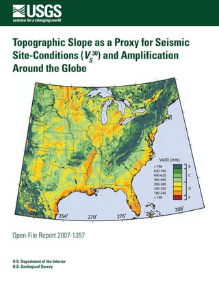
  • 15. Figure 1. A, The topographic relief map for the State of California with elevation in meters (see legend). B, Site-condition map for California based on geology and VS observations (modified from Wills and others, 2000). C, Site-condition map derived from topographic slope using the correlations indicated in table 2. 8
  • 16. Figure 2. Correlations of measured VS 30 (m/s) versus topographic slope (m/m) for A, active tectonic, and B, stable continental regions. Color-coded polygons represent VS 30 and slope ranges consistent with ranges given in table 2 and also consistent with the VS 30 legends for all geologic- and topographic-based maps throughout this paper. Figure 3. Histograms indicating logarithmic differences of measured Californian VS 30 values compared with A, values derived from topographic slope correlations and, B, values based on existing VS 30 site-condition maps. N is the number of VS 30 measurements. 9
  • 17. 10
  • 18. Figure 4. A, Topographic map of the San Francisco Bay Area. Circles indicate the location of measurements, color-coded by VS 30 in m/s (see left legend). B, Site-condition map based on geology and VS 30 observations (modified from Wills and others, 2000). C, Site-condition map derived from topographic slope. D, The ratio of the predicted amplification for a uniform PGA of 250 cm/s2 for the geologically- and topographically-based VS 30 maps. Blues indicate that the Wills and others (2000) map predicts higher amplification, whereas reds indicate higher amplifications are predicted from the topographically-based map. White indicated where the two VS 30 maps predict the same amplification. 11
  • 19. Figure 5. A, Topographic map of the Los Angeles region. Circles indicate the location of measurements, color-coded by VS 30 in m/s. B, site-condition map based on geology and VS 30 observations (modified from Wills and others, 2000). C, Site- condition map derived from topographic slope. D, The ratio of the predicted amplification for a uniform PGA of 250 cm/s2 for the geologically- and topographically-based VS 30 maps. 12
  • 20. Taiwan The next question we address is whether the correlations hold in areas that have similar overall topographic expression but exhibit different geology, tectonics, and geomorphology. Taiwan was chosen to test this hypothesis, primarily because the site classes on a national scale are well-understood from prior studies (for example, Lee and others, 2001) and are available for direct comparison. The high seismicity in Taiwan results from the convergence of the Philippine Sea plate and the Eurasian plate. The Philippine plate is moving NW at a rate of about 7 cm/yr relative to the Eurasian plate. The abundance of shear-wave observations used in our correlations provides us with a valuable validation case study to ensure that the slope calibration with VS 30 is robust among our base data sets. Figure 6 shows the topographic map superimposed with color-coded VS 30 measurements (fig. 6a), the national site-condition map (fig. 6b; modified from Lee et al., 2001), and the topographic-gradient derived VS 30 map for the island of Taiwan (fig. 6c). Shallow shear-wave velocities around Taiwan vary widely, but they do so with rather systematic trends that are well-recovered using topographic slope. Figure 7a provides the ratio of measured versus slope-derived VS 30 values. The mean and standard deviation are comparable to those evaluated for California sites (fig. 3a). In presenting the Taiwanese site-condition map, we have assigned median shear velocities based on the NEHRP categories adopted by Lee and others (2001), the exception for this being site class E, where we assigned a VS 30 of 150 m/s. Statistically, the topographically-derived site-condition map for Taiwan performs very well (fig. 7a) relative to the geologically-based map (fig. 7b). The Taiwanese are currently working on a revised site classification scheme that should further improve comparisons to measured data (C.-T. Lee, written commun., 2007). The correlations derived jointly from California and Taiwan shear-wave observations and topographic slope seem to apply in areas of similar overall topographic expression independent of other factors that may be contributing. It is interesting to note that, in a significant number of the examples represented in this report, population exposure tends to correlate very well with slower VS 30 site-conditions calculated from the slope of topography. Intuitively, the correlation between population density and seismic site-condition is not surprising since steep hill slopes are not usually as desirable for building structures, while flat-to- gently sloping lands tend to consist of more fertile soils suitable for agricultural purposes and have traditionally been inhabited. Using Taiwan as an example, we compare seismic site-condition to population exposure as derived from the Oak Ridge National Laboratory’s LandScan 2005 database (Dobson and others, 2000; Bhaduri and others, 2002) (fig. 6d). We see that urban communities appear to be most dense in the flat-lying lands that correspond to lower VS 30 . In particular, the region around Taipei possesses significant amplification potential owing to its location on primarily NEHRP site class D surficial material. Population becomes less dense as we grade from gently sloping to steeper terrains. This figure serves to remind urban planners, disaster mitigators, and emergency responders why we must consider seismic site-conditions as an important component in earthquake hazard assessment, since those areas with the densest populations are also likely to have the strongest site amplifications. 13
  • 21. 14
  • 22. Figure 6. A, Topographic map of Taiwan with elevation in meters. Circles indicate the location of measurements, color- coded by VS 30 in m/s. B, Site-condition map based on geology and VS 30 observations (modified from Lee and others, 2001). C, Site-condition map derived from topographic slope. D, Population density map of Taiwan derived from the LandScan 2005 population database (for example, Dobson and others, 2000; Bhaduri and others, 2002). See figure 1 for topography and VS 30 legends. Figure 7. Histograms indicating logarithmic differences of measured Taiwanese VS 30 values compared with A, values derived from topographic slope correlations and, B, values based on existing VS 30 site-condition maps. N is the number of VS 30 measurements. Differences in N between A and B arise when the grid point referred to is not defined within the selected map grid. Alaska Alaska is the most seismically active state in the United States, largely because of the active subduction of the Pacific plate beneath the North American plate at a rate of about 5–7 cm/yr. The region has hosted two great-magnitude (M > 9.0) earthquakes since 1957 along this tectonic plate boundary (Wesson and others, 1999). In addition to earthquakes occurring along the subduction zone, significant seismicity also occurs throughout Alaska as a result of stresses imposed by interaction of the plates. Much of this relative motion is accommodated at the principal boundary between the two plates in the Gulf of Alaska, but there is also substantial crustal deformation and earthquake activity inland of the plate boundary in central Alaska. In addition to occurring on major mapped faults such as the Denali fault, shallow-focus earthquakes in central Alaska also occur on lesser, unmapped faults. Many studies have been undertaken that examine site response within Anchorage, given its high seismic hazard, relatively high exposure, and geographic setting within a sedimentary basin (for example, Nath and others, 1997; Dutta and others, 2000; Combellick, 2001; Dutta and others, 2001; Martirosyan and others, 2002; Dutta and others, 2003; Badal and others, 2004). Indeed, ground failure in Anchorage following the 1964 Prince William Sound earthquake was widely reported (Martirosyan and others, 2002; Dutta and others, 2003). Such studies, however, are only available on a very localized scale. A state wide site-condition map for Alaska has been developed by Martirosyan and Hansen (2007) for use in ShakeMap applications. However, this map was unavailable for comparison at the time this report was written. 15
  • 23. We generate a VS 30 map for the State of Alaska using our topographically based approach. In general, we observe that much of the southern margin of the state, adjacent to the subduction zone, indicates relatively fast material, consistent with the dynamic topographic relief (fig. 8). Another feature that can clearly be identified in our VS 30 map of Alaska is the Yukon delta in western Alaska. This region indicates slower-velocity surficial material consistent with fluvial processes of the Yukon River. Also of note in figure 8 is the low velocity of the braided river systems throughout the Mackenzie River Basin in northwestern Canada. Next we investigate the seismic site-conditions of Anchorage in more detail and superimpose combined VS 30 values from Dutta and others (2000) and the PEER NGA database (fig. 9a). Despite the limited resolution, much of Anchorage indicates lower-velocity surficial materials (fig. 9b) consistent with the city’s location within a sedimentary basin. In general, our result is consistent with the more detailed studies in Anchorage mentioned above, with mapped VS 30 grading from fast to slower velocities westward towards the harbor. Statistically, our predictions of VS 30 compare very well with observed VS 30 values at strong-motion sites across Alaska and with measurements taken in Anchorage (fig. 10). 16
  • 24. Figure 8. A, The topographic relief map for the State of Alaska. B, Site-condition map derived from topographic slope. 17
  • 25. Figure 9. A, Topographic map of the Anchorage, Alaska region. Circles indicate the location of VS 30 measurements, color- coded by velocity in m/s. B, Site-condition map derived from topographic slope. See figure 1 for figure legends. Figure 10. Histogram indicating logarithmic differences of combined Anchorage (Dutta and others (2000) and NGA VS 30 values compared with values derived from topographic slope correlations. 18
  • 26. Nevada Scott and others (2004) describe the collection of VS 30 data on a transect along the Truckee River in Reno, Nevada. These results, based on microtremor analysis, suggest that VS 30 is higher than that expected from alluvium-filled basins, based on NEHRP previsions. Scott and others, (2004) concluded that mapped surficial geology is not necessarily a reliable predictor of VS 30 , owing to stiffer underlying Tertiary sediments. The location of this survey, closely following an erosive river environment, may be a possible explanation for these results. Consequently, we observed that the Nevada data indicated systematically higher velocities with topographic slope than our reference dataset for California and Taiwan. We use no data from Nevada in our correlations between slope and VS 30 . A local adjustment factor may have to be applied to the VS 30 map based on topographic slope. We have not developed a separate topographic slope-based map for the State of Nevada. However, the State is largely represented in the northeast quadrant of the California map (fig. 1). Site classifications for Nevada appear to be highly variable, with spatially periodic changes in site class that are associated with the Basin and Range tectonic province (fig. 1c). Salt Lake City, Utah The next example within active tectonic regions is that of the Salt Lake City, Wasatch Front region of Utah. This site-condition map can also be considered a forward prediction since, unlike California and Taiwan, no VS 30 data for this region were used in our calibration analysis. The data, which were obtained from the Utah Geological Survey, appeared to have VS 30 values systematically lower than mean values from other active regions with similar slope (fig. 2a). The geologically- and topographic slope-based maps (figs. 11b and 11c, respectively) demonstrate similar trends. However, there appears to be a significant trend towards lower velocities in the geologically-based site map, west of the Wasatch Front. This observation is consistent with the measured data. On average, the geology- based map (fig. 12b) represents the measured data better than does the slope-derived map (fig. 12a). The latter shows an overall bias indicating that VS 30 predictions in the Salt Lake City region are on average over-predicted by the topographic-slope approach employing the current correlations. It is possible that near-surface shear velocities in the region are lower for a given slope angle than in California and Taiwan, and thus require slight modification to the slope versus VS 30 correlation. Alternatively, the VS 30 measurements underestimate actual in situ velocities for some other reason, not yet established. While we observe that the slope-derived map (fig. 11c) indicates a more natural progression of VS 30 grading towards higher values in steeper topographic relief, it is also possible that Lake Bonneville deposits that abut the mountain front, rather than sloping, may violate the basic assumption on which our correlations are based (K. Pankow, written commun., 2007). The small overall bias in the Salt Lake City region could be removed with an overall shift of about 25 percent in predicted VS 30 values, though it is possible that these biases are concentrated in particular geological units. 19
  • 27. Figure 11. A, Topographic map of the Salt Lake City, Wasatch Front region of Utah. Circles indicate the location of measurements, color-coded by VS 30 in m/s. B, Site-condition map based on geology and VS observations. C, Site- condition map derived from topographic slope. 20
  • 28. Figure 12. Histograms indicating logarithmic differences of measured Utah VS 30 values compared with A, values derived from topographic slope correlations and, B, values based on existing VS 30 site-condition maps. N is the number of VS 30 measurements. Seattle, Washington The Cascadia subduction zone lies just off the coast of Oregon and Washington. This subduction zone is the main tectonic feature in the geologically active Pacific Northwest. On shore, the (continental) North American plate overlays the subducting (oceanic) Juan de Fuca plate. Assessment of the regional shaking impact of an anticipated great Cascadia subduction zone earthquake requires at least a first-order approximation of site-conditions. The contribution of site response to the observed ground shaking is well recognized in the Seattle region (Frankel and others, 1999). Assessment of site characteristics has found that sites on artificial fill are likely to experience significant response from an input ground motion. Given that no Seattle data were used in the model development, our topographically-based assessment of VS 30 can be considered as forward prediction of seismic site-conditions. Visually, the topographically-based map appears to recover many of the key features in the geology-based map (figs. 13b and 13c). The former does indicate greater variability in predicted VS 30 than the latter, particularly in the lower-lying regions to the southwest of downtown Seattle, where a higher proportion of slower D class material is predicted. However, the geologically-based map predicts more slow E class material. The topographic approach also predicts more higher-velocity B class material within the mountains that bound the city. Statistically, the topographically-based map represents the observed values relatively well (fig. 14a) however, there is not a strong correlation. The geologically-based map has a strong peak about the median value consistent with the fact that it was based on these observed VS 30 values (fig. 14b). These results suggest that VS 30 maps based on topography alone can serve as a suitable proxy in the absence of more detailed geologically-based site-condition maps. 21
  • 29. Figure 13. A, Topographic map of the Seattle, Washington, region. Circles indicate the location of measurements, color- coded by VS 30 in m/s. B, Site-condition map based on geology and VS observations. C, Site-condition map derived from topographic slope. 22
  • 30. Figure 14. Histograms indicating logarithmic differences of measured Seattle, Washington VS 30 values compared with A, values derived from topographic slope correlations and, B, values based on existing VS 30 site-condition maps. N is the number of VS 30 measurements. Indonesia The origin of the Indonesian Archipelago about the Sunda Arc results from the active subduction of the Indo-Australian tectonic plate beneath the Eurasian plate. The high rate of destructive seismicity that accompanies this plate motion has been recently demonstrated by several catastrophic earthquakes including the 2004 MW 9.0 and 2005 MW 8.7 Sumatra-Andaman Islands earthquakes, and the 2006 MW 6.3 Yogyakarta earthquake. Little information regarding the response of near-surface geology to strong ground shaking in Indonesia is available. However, a reconnaissance report following the 2006 Yogyakarta earthquake notes that the most heavily damaged areas were underlain by young volcanic deposits consisting of undifferentiated tuff, ash, breccia, agglomerates, and lava flows (Earthquake Engineering Research Institute, 2006). Moreover, the report explicitly states that the most pronounced effects were associated with directivity and soil amplification. Consequently, first-order estimates of seismic site-conditions for Indonesia will be important to assess earthquake hazard in future studies. A pilot hazard study performed in the Sulawesi Province also suggested significant potential for ground motion amplification owing to effects of surficial geology (Thenhaus and others, 1993). Figure 15a shows the topographic relief of Indonesia. Because of the active subduction of the Indo-Australian plate beneath the island arc, the topographic signature of the islands is dominated by a chain of active volcanoes adjacent to the subduction zone. The margin most distant from the active subduction indicates more subdued topography grading to relatively flat slopes near the coastlines. This subdued topography is particularly apparent for the island of Sumatra. The corresponding VS 30 map derived from the slope of topography (fig. 15b) indicates broad regions of low-velocity surficial materials (NEHRP site class D). The steeper volcanic chain is indicated by faster BC to B surficial materials. We also note narrow zones of lower VS 30 along the margins nearest the Sunda Arc. Figure 15c shows the population density map for Indonesia, one of the most densely populated nations on Earth. The island of Java is particularly heavily populated, with much of the exposure correlating to NEHRP site classes C and D. High exposure rates are also observed in southeastern Sumatra, which again is largely mapped as site class D. 23
  • 31. 24
  • 32. Figure 15. (Facing page) A, Topographic map of Indonesia. B, Site-condition map derived from topographic slope. C, Population density map of Indonesia. See figure 6 for map legends. Iran This highly seismic region forms the north-west trending boundary between the Arabian and Eurasian tectonic plates. The Arabian plate is a small plate split from the African plate by rifting along the Red Sea. As it underthrusts the Eurasian Plate it causes uplift of the Zagros Mountains and numerous devastating earthquakes. Iran has suffered many deadly earthquakes in the recent past with death tolls in excess of 1000 each; for example 1962 MS 7.3 Buyin-Zara; 1968 MS 7.3 Dasht-e Bay z; 1972 MS 6.9 Ghir; 1976 MW 7.0 Iran-Turkey border; 1978 MW 7.3 Tabas; 1981 MW 7.2 Sirch; 1990 MW 7.4 Manjil; 1997 MW 7.2 Ardakul; and 2003 MW 6.6 Bam. The combination of high hazard and primarily poorly constructed adobe structures makes Iran an extremely high-risk region. In almost all of the earthquakes noted above, it was identified that adobe houses located on alluvium suffered greater damage than those located on firm gravels or rock sites (Ambraseys, 1963; Bayer and others, 1969; Dewey and Grantz, 1973; Berberian, 1979; Berberian and others, 1992; Jafari and others, 2005; Building and Housing Research Center, 2007). Consequently, first-order estimates of seismic site-conditions are fundamental for quantifying regions at risk for strong ground shaking from surficial effects. We superimpose some significant Iranian earthquakes listed above onto the topographic map (fig. 16a). From the seismic site-condition map developed from the slope of topography, we observe that many of these deadly earthquakes have occurred near sites of relatively low VS 30 (fig. 16b), consistent with our earlier observation that populations tend to concentrate on flat-lying sedimentary basins. In particular, the deadly Manjil earthquake near the Caspian Sea, which resulted in approximately 35,000 deaths (Utsu, 2002), is located in close proximity to large Quaternary sedimentary deposits, indicated by low VS 30 in figure 16b (for example, Niazi and Bozorgnia, 1992). The Dasht-e Bay z and Bam earthquakes, which resulted in very high casualties (15,000 and 26,000 deaths, respectively), also occurred near regions of significant amplification potential, and this is likely to have contributed to the extreme number of fatalities observed. Unfortunately, no VS 30 measurements are available from Iran for comparison. 25
  • 33. 26
  • 34. Figure 16. (Facing page) A, Topographic relief map for Iran, superimposed with the epicenters of recent deadly earthquakes (red stars). B, Site-condition map derived from topographic slope. Italy Primary tectonic activity in Italy results from the collision of the Eurasian and African Plates. The high-topography zone of the central Apennines, which trends NW-SE within peninsular Italy, is dissected by a Quaternary fault system that has hosted several moderate-to-large historical earthquakes (Cello and others, 1997), most recently 1980 MW 6.9 Iripinia, and 1997 MW 6.0 Umbria-Marche. Site response effects were documented following the 1997 Umbria-Marche seismic sequence (Caserta and others, 2000; Tertulliani, 2000). In 2002, the Molise and Puglia regions of southern Italy were struck by two moderate-magnitude earthquakes (Cara and others, 2005). The first and largest of the two (MW 5.7) resulted in 30 casualties in the town of San Giuliano di Puglia. The high intensities observed in this town are largely attributed to local site-conditions (Cara and others, 2005). The Istituto Nazionale di Geofisica e Vulcanologia (INGV), Italy, has recently installed the ShakeMap system as a routine process of its national earthquake monitoring program. We obtained the national site-condition map that is used in this system (fig. 17b) courtesy of A. Michelini (written commun., 2006). In general, the topographically-derived map (fig. 17c) demonstrates many of the same features as the geologically-derived map. However, there are some discrepancies over the absolute value of VS 30 assignments. We observe that the geologically-based map (fig. 17b) has systematically higher velocities than our topographically-based map (fig. 17c). This difference is reflected in figure 18 when we compare VS 30 values at Italian strong-motion stations, available from the PEER NGA project, with the respective site-condition maps. Despite a larger spread in the comparisons, the topographically-based map tends to recover individual VS 30 values better than the geologically-based map, which is biased towards higher velocities. Again, population density correlates well with flat- lying, low-VS 30 areas (fig. 17d). Although the site-condition maps generally indicate similar trends, one obvious disparity between them occurs in the Puglia region of southeastern Italy, where figure 17b indicates significantly faster velocities than are predicted by the topographic approach. The predominant geology comprises flat-lying Mesozoic shallow-water carbonate and evaporite rocks (de Alteriis and Aiello, 1993). Relative to much of Italy and other Mediterranean regions, the seismicity of Puglia is quite low. This observation is subsequently reflected in the absence of significant topographic relief. Consequently, we can conclude that, in geological conditions dominated by these flat-lying carbonates, the automated topographic approach may not recover VS 30 as well as a more rigorous assessment of local surficial geology. 27
  • 35. Figure 17. A, Topographic map of Italy. Circles indicate the location of measurements, color-coded by V 30 S . B, Site- condition map based on geology and VS observations. C, Site-condition map derived from topographic slope. D, Population density map of Italy. See figures 1 and 6 for map legends. 28
  • 36. Figure 18. Histograms indicating logarithmic differences of Italian VS 30 values from the NGA dataset, compared with A, values derived from topographic slope correlations and, B, values based on existing VS 30 site-condition maps. N is the number of VS 30 measurements. Japan Japan is a densely populated nation that is high in seismic hazard. Much of Japan’s population resides on thick sedimentary basins that have significant potential to amplify ground shaking. Tectonically, Japan is located near the junction of the Pacific, Philippine Sea, and Okhotsk tectonic plates. The Pacific plate is moving northwest at a rate of about 8–9 cm/yr relative to, and subducting beneath, the Philippine Sea and Okhotsk plates. In addition, the Philippine Sea plate is subducting northward beneath Japan and the Okhotsk and Amurian plates (Miller and Kennett, 2006). The complex tectonics drive the high rates of seismicity observed in the region, and the subducting slabs provide the source for the many active volcanoes that occupy the island. Figure 19a shows the topographic map of Japan. We have obtained a geologically-based VS 30 map (fig. 19b) of Japan courtesy of M. Matsuoka (written commun., 2006). This map was developed analyzing geomorphic characteristics tied to VS 30 measurements (Matsuoka and others, 2005). They further refine this model using multiple linear regression analysis on additional geomorphic indicators; i.e., correlating VS 30 with elevation, topographic slope, and the distance from mountain ranges. Our purely topographically-based map (fig. 19c) exhibits many of the same trends as the Matsuoka and others (2005) map. However, the topographic approach does not predict as much slow-velocity material (equivalent to NEHRP site class E) as indicated in figure 19b. As with Taiwan, we also plot the population exposure (fig. 19d) and compare this with the site-condition map. Again we note a strong correlation between population density and assignments of low VS 30 . Shallow shear-wave velocities have been determined for a number of sites within the KiK-Net strong-motion network (Kawase and Matsuo, 2004; H. Kawase, written commun., 2006). Kawase and Matsuo (2004) made these VS 30 estimates by first using a spectral inversion of ground motion recordings to determine site factors, and then inverting for the best fit 1-D shear-velocity model using a genetic algorithm. Unlike most other regions studied, many of these sites were located on rock, so the distribution is biased towards higher-velocity VS 30 data. The ratio of measured VS 30 to predicted VS 30 is 29
  • 37. compared for both site-condition maps in figure 20. We observe no significant difference between the geologic- and geomorphic-based map of Matsuoka et al. (2005) and our site-condition map based on topographic slope. However, it appears that both maps tend to underestimate VS 30 , relative to observed data. We note that there is not uniform sampling of VS 30 data across all possible site classes, with only a limited number of C and D site classes available for comparison. Furthermore, this strong-motion network was probably designed so that the accelerometers were located at “hard rock” sites. Consequently, it is expected that the location of these sites will be more biased towards faster velocities than average sites of similar topographic slope. Since these VS 30 values were not derived from more widely used measurement techniques, we are as yet unsure of the consistency of this approach compared with more standard VS 30 measurements; however, the strong correlation of the two VS 30 maps (figs. 19B, C) with each other provides some level of confidence in the overall results. Also, as noted earlier, the differences between observed and topographically-based VS 30 may not affect amplification potential significantly since most of the data are of higher velocity, which occurs near or above the BC boundary and where site effects are not as pronounced. 30
  • 38. 31
  • 39. Figure 19. A, Topographic map of Japan. Circles indicate the location of VS 30 measurements, color-coded by velocity in m/s. B, Site-condition map based on geology and VS 30 observations (modified from Matsuoka and others, 2005). C, Site- condition map derived from topographic slope. D, Population density of Japan. Figure 20. Histograms indicating logarithmic differences of Japanese VS 30 values, compared with A, values derived from topographic slope correlations and, B, values based on existing VS 30 site-condition maps. N is the number of VS 30 measurements. The difference in N between the two histograms is because some of the VS 30 measurement points are plotted outside the grid defined by the geologic- and geomorphic-based map of Matsuoka and others (2005). Mexico One of the most obvious and most well-documented occurrences of seismic site amplification resulted from the great 1985 MW 8.1 Michoacan earthquake that devastated Mexico City, some 350 km from the epicenter (for example, Campillo and others, 1989; Glass, 1989; Ordaz and Singh, 1992). In this case, a number of factors contributed to the high damage rates observed, including complex heterogeneous rupture (Campillo and others, 1989), enhanced transmission path (Furumura and Kennett, 1998), basin resonance effects at long periods (2–3 sec), and local site response from lakebed sediments (Campillo and others, 1989). Much of Mexico’s seismicity is driven by the subduction of the Rivera and Cocos microplates beneath the Pacific coast of Mexico (part of the North American plate). The slower subducting Rivera Plate is moving northeast at about 2 cm/yr relative to the North American plate, and the faster Cocos plate is moving in a similar direction at a rate of about 4.5 cm/yr. These microplates interact with the larger Pacific plate via a combination of transform faults and spreading ridges (DeMets and Stein, 1990). Further north, the Gulf of California represents a developing transform-rift margin (Umhoefer and others, 1994). We calculate a VS 30 map for the country of Mexico from the topographic slope employing the coefficients for active tectonic regions (fig. 21). We observe that relatively high VS 30 values are associated with the Sierra Madre Occidental and Oriental mountain ranges along the western and eastern margins of the Mexican Plateau, respectively. The Mexican Plateau itself is represented by more complex VS 30 patterns, but in general is indicated by slower surficial materials relative to the mountain ranges that bound the plateau. The surficial materials that make up the Mexican Plateau are 32
  • 40. most likely weathering products derived from the Sierra Madre Mountains via fluvial processes. Slower velocity materials are also predicted along the western coast of Mexico along the Gulf of California and Pacific coastlines. Again, these surficial materials are most likely derived from weathering processes within the Sierra Madre Occidental Mountains. Figure 22 shows a more detailed view of the seismic site-conditions about Mexico City. Much of the city is built upon lakebed sediments, which are known to have contributed to seismic wave amplification following the devastating 1985 Michoacan earthquake (Ordaz and Singh, 1992). The topographically-based VS 30 map indicates that much of Mexico City is built upon NEHRP site class D. The extent of site class D also corresponds to the regions of highest population density (fig. 22c). Figure 21. VS 30 map for Mexico employing the coefficients for active tectonic regions. See figure 22 for a more detailed view of Mexico City. 33
  • 41. Figure 22. A, Topographic relief map of Mexico City. B, Site-condition map derived from topographic slope. C, Population density map of Mexico City. New Zealand New Zealand straddles the boundary between the Indo-Australian and Pacific tectonic plates. The relative plate motion in New Zealand is expressed by a complex assemblage of active faults, coupled with a moderately high rate of seismicity (Stirling and others, 2002). The plate boundary beneath New Zealand comprises the Hikurangi (North Island) and Fiordland (far south of South Island) subduction zones, which dip in the opposite sense relative to each other. Active tectonic motion is accommodated by the faults of the axial tectonic belt that traverse much of the South Island between the subducting slabs (Stirling and others, 2002). The Alpine Fault in the central South Island accommodates the release of much of the strain energy produced by the relative plate motion. 34
  • 42. Significant site response effects have been observed from several of New Zealand’s large earthquakes. Furthermore, microzoning was clearly recognized following the deadly M 7.8 1931 Hawke’s Bay earthquake. Dowrick and others (1995) note that the structures most affected by this earthquake were located on rock sites and the least damage occurred on the soft alluvium sites. They conclude that topographic effects may have enhanced the ground shaking in rock locations, and strong ground shaking at high frequencies was attenuated on the deep basin sediments. In contrast to these observations, Abercrombie and Benites (1998) noted that weak-motion data recorded in the cities of Hastings and Napier, both of which were affected by the 1931 quake, exhibited prolonged duration and amplification of shaking owing to the existence of thin soil layers above a Miocene-age sedimentary basin. These data suggest that there may be strong nonlinear behavior of the soils in this region when subjected to increasing levels of ground shaking. More recently, a reconnaissance report following the MW 6.5 1987 Edgecumbe, Bay of Plenty earthquake indicated that most of the damage occurred on drained swampland consisting of soft, unconsolidated soils (EQE Incorporated, 1987; Franks, 1988). Based on these observations, it is important that the effects of site response should be considered for hazard and risk assessments in regions such as New Zealand. Based on our topographic approach for defining seismic site-conditions, we observe that many of New Zealand’s most developed urban centers appear to be located in regions of significant amplification potential, including Greater Wellington, Christchurch, Hastings, Napier, Dunedin, and Invercargill (figs. 23 and 24). Limited work in defining VS 30 in the Greater Wellington region has been performed through collaborations among the University of Nevada, Reno; Victoria University, Wellington; and the Institute of Geological and Nuclear Sciences (see http://www.seismo.unr.edu/ hazsurv/#wnlh). This work culminated in approximately 90 VS 30 measurements across the local area, from the city of Wellington to Upper Hutt. We compare our topographically-based map of the Wellington region with these measured values (fig. 25). Despite limitations in the resolution of the topographic data and the tight spatial clustering of the VS 30 measurements, we observe the same general trends are recovered by the topographic-based site-condition map. This dataset, however, comprises more E site class material than is predicted with the topographic approach. The availability of higher-resolution topography data in this region may yield site-conditions more comparable to the observed data. 35
  • 43. Figure 23. A, Topographic relief map for New Zealand’s North Island. B, Site-condition map derived from topographic slope. 36
  • 44. Figure 24. A, Topographic relief map for New Zealand’s South Island. B, Site-condition map derived from topographic slope. See figure 23 for map legends. Figure 25. A, Topographic map of the Greater Wellington region, New Zealand. Circles indicate the location of measurements, color-coded by VS 30 (see figure 23). Data were measured through collaborations between the University of Nevada, Reno; Victoria University, Wellington; and the Institute of Geological and Nuclear Sciences. B, Site-condition map derived from topographic slope. See figure 23 for map legends. 37
  • 45. The Philippines The Philippine archipelago represents a complex system of microplates that are being compressed between two convergent plate margins that bound the nation: the Philippine Sea and Eurasian plates. Because of its tectonic setting, the Philippines experiences frequent damaging seismic activity. It was reported following the MW 7.7 1990 Central Luzon earthquake that the most serious damage occurred on soft soil sites (EQE Engineering, 1990). The seismic site-condition map for the Philippines, derived from topographic slope, indicates several broad regions of low VS 30 (fig. 26b). Slower VS 30 values generally tend to mimic the regions of highest population exposure (fig. 26c). Consequently, site response will be an important factor when providing rapid estimates of ground shaking following a large earthquake in the region. 38
  • 46. Figure 26. A, Topographic map of the Philippines. B, Site-condition map derived from topographic slope. C, Population density map of the Philippines. Puerto Rico The island of Puerto Rico, in the northwest Caribbean, lies within a broad deformation zone between the Caribbean and North American tectonic plates (Masson and Scanlon, 1991). In 1999, the USGS held a workshop to develop strategies to mitigate against earthquake and tsunami hazards in the region (Brink and others, 1999; Mueller and others, 2003). One of the key outcomes from this workshop was the need to develop a site response map for Puerto Rico. Puerto Rico has recently installed the ShakeMap system (Clinton and others, 2006) that incorporates a national site-condition map (fig. 27b). This map is based upon VS 30 measurements conducted by Odum and others (2007). We compare the topographically-derived site-condition map (fig. 27c) with the map based on geology and VS 30 measurements (fig. 27b). The first thing that is apparent from figure 27b is the absence of any significant lateral variability in VS 30 assignments. Except for minor variations along coastlines and tributaries, existing ShakeMap VS 30 site-conditions are mapped almost entirely between 360–490 m/s. The topographically-derived map, however, demonstrates significant variability, and 39
  • 47. mapped extents appear consistent with the mapped geology where harder plutonic and volcanic rocks are recovered with fast VS 30 , while Quaternary alluvial deposits are recovered with slower VS 30 (see Fig. 2 in Odum and others, 2007). The number of VS 30 measurements are limited for the island of Puerto Rico. However, we use data from two recent studies (Pérez-Marcial, 2005; Odum and others, 2007) to evaluate both site- condition maps. We find a good correlation between measured VS 30 and predicted VS 30 from the topographic slope method (fig. 28a). The geologically-based map, however, appears to be a very poor predictor of VS 30 (fig. 28b). Figure 27. A, Topographic map of Puerto Rico. Circles indicate the location of measurements, color-coded by VS 30 in m/s. B, Site-condition map based on geology and VS observations. C, Site-condition map derived from topographic slope. 40
  • 48. Figure 28. Histograms indicating logarithmic differences of Puerto Rican VS 30 values from Pérez-Marcial (2005) and Odum and others (2007), compared with A, values derived from topographic slope correlations and, B, values based on existing VS 30 site-condition maps. N is the number of VS 30 measurements. Turkey Turkey is a tectonically active region that experiences frequent destructive earthquakes. First- order tectonics are controlled by the collision of the Arabian plate and the Eurasian plate. A large piece of continental crust almost the size of Turkey, called the Anatolian block, is being compressed in a westerly direction. The block is bounded to the north by the North Anatolian Fault and to the southeast by the East Anatolian Fault. It was observed following the deadly 1999 zmit earthquake that site effects were a significant contributor to the high human losses (Bray and Stewart, 2000; Rathje, 2000; Bakır and others, 2002). We compare the national site-conditions map for Turkey compiled by Department of Earthquake Engineering, Kandilli Observatory and Earthquake Research Institute (KOERI; Z. Cagnan, written commun., 2007), derived from geologically-based data (fig. 29b), with our topographically- derived map (fig. 29c). The former was prepared using the correlations of NEHRP site classifications as a function of lithologic age, as described by Wills and Silva (1998). From this work, Turkey was assigned three different site classes: B, C, and DE. We assign VS 30 to the Turkish geologically-based map by taking the median NEHRP value for classes B and C, while the DE site class was assigned on the basis of the range given by Wills et al. (2000). The topographic-slope technique recovers most of the features indicated by the geology-based approach. Shear-wave values obtained from the NGA dataset are compared to the topographically-based approach (fig. 30a). In general, the topographic slope method tends to overestimate VS 30 with respect to the values given in the NGA database. However, there are reservations over the quality of these assignments since they were not derived from in situ measurement techniques. The same comparison using the Turkish national site-condition map appears to overestimate VS 30 as well, but yields a better overall median value with a slightly higher standard deviation (fig. 30b). 41
  • 49. 4242
  • 50. Figure 29. A, Topographic map of Turkey. Circles indicate the location of measurements, color-coded by VS 30 in m/s. B, Site-condition map based on surficial geology from KOERI (Z. Cagnan, written commun., 2007). C, Site-condition map derived from topographic slope. See figure 1 for map legends. Figure 30. Histograms indicating logarithmic differences of Turkish VS 30 values taken from the NGA database, compared with A, values derived from topographic slope correlations and, B, values based on existing VS 30 site-condition maps. N is the number of VS 30 measurements. Southern Europe The moderate-to-high rate of seismicity in the Mediterranean region originates from the convergence of the African and Eurasian tectonic plates at a rate of about 6 mm/year. To date, little work available to the public has been done to constrain parameters for regional site-conditions. Using the active tectonic VS 30 -slope relations (fig. 31), we observe that many features of the southern European and northern African geologic landscape are well recovered using our technique. Major mountain belts are clearly identified as high velocity zones, including the Alps, Pyrenees (France and Spain), Apennines (Italy), Dinaride (Greece), and Atlas (Morocco, Algeria, and Tunisia) mountain ranges. Other features such as the Po Basin (Italy) and Nile River Delta (Egypt) are clearly identified as low velocity zones. Less obvious at this scale, the Rhône (France) and Rhine (France and Germany) River Valleys can also be identified as a low seismic velocity zone. 43
  • 51. Figure 31. A, Topographic relief map for Southern Europe, Anatolia, and Northern Africa. B, Site-condition map derived from topographic slope. See figure 1 for map legends. 44
  • 52. Application in Intraplate Regions Mississippi Embayment Region As expected from basic geomorphology, in areas of significant relief, mountains correlate well with rock and basins correlate well with sediments. Will this approach work in areas of lower overall relief? While a similar range of shear-velocity measurements, from hard rock to soft sediments, exist in the Mississippi Embayment, the associated topography as captured by the 30 arc sec (approximately 1 km resolution) SRTM30 data is much more subdued, as indicated by the narrow range in elevation (fig. 32a). Hence, there is less variation in slope and consequently, it might be expected that it would be more difficult to assign slope ranges that define the VS 30 categories. Furthermore, as in the active tectonic regions, few VS 30 measurements are available for high-velocity, hard rock sites. Nonetheless, there does appear to be a natural progression among VS 30 values plotted against slope for both the central Australia and United States (fig. 2b), and we use these limits to produce the slope-based site-condition map for the Mississippi Embayment region shown in figure 32. We compare the 432 VS 30 measurements with topography (fig. 29a), the VS 30 site-condition map (fig. 32b) used for the regional ShakeMap installation (Bauer and others, 2001; Brackman, 2005), and the slope-derived VS 30 map (fig. 32c) at sites in the Mississippi Embayment. We find excellent correspondence of measured and slope-estimated VS 30 values. The lowest VS 30 regions, particularly those along river channels and in the Mississippi Embayment itself, are recovered, as are the few relatively high-velocity VS 30 values in the southwestern corner of the map. On average there is very little bias to the estimates (fig. 33a). The same cannot be said of the geology-based site- condition map (fig. 32c), which shows an overall bias, having significantly lower VS 30 values with respect to those measured (fig. 33b). Likewise, there is a more continuous progression of varying VS 30 in the topography-based map (fig. 32c) than in the geology-based map (fig. 32b). Furthermore, the current map shown in figure 32b, used by the Central United States Earthquake Consortium (CUSEC), itself shows significant inconsistencies across state borders because they were mapped independently by different researchers. These inconsistencies are mostly observed outside the embayment itself. Consequently, it appears that the slope versus VS 30 categories for this region of low topographic relief can successfully be used as a proxy for basic site-conditions, just as for tectonically active regions. Another redeeming feature is that either the slope range or the mean slope values for a given region can provide simple quantitative diagnostics for the nature of the appropriate VS 30 -slope coefficients applied to the region. For example, mean slope values for the active tectonic regions are about 0.07; for the Mississippi Embayment region the mean slope is much lower, at 0.01, and over the entire continental United States east of the Rocky Mountains, the slope mean is about 0.04. Hence, we can use the mean slope to establish which slope correlations should be employed: active tectonic or stable continent. Alternatively, simplified characterizations of tectonically active versus stable continent domains could suffice in choosing between the coefficients employed for slope-based VS 30 assignments. 45
  • 53. Figure 32. A, Topographic map showing the Mississippi Embayment region of the central United States. Circles indicate the location of measurements, color-coded by VS 30 in m/s. B, Site-condition map based on geology and VS observations (modified from Bauer and others, 2001). C, Site-condition map derived from topographic slope. 46
  • 54. Figure 33. Histograms indicating logarithmic differences of VS 30 values for the Mississippi Embayment region, compared with A, values derived from topographic slope correlations and, B, values based on existing VS 30 site-condition maps. N is the number of VS 30 measurements. Australia Despite Australia’s stable continental setting, it has hosted several large earthquakes in the past 50 yrs (for example, McCue, 1990; Clark and McCue, 2003). In contrast to most stable continental regions, where the largest magnitude earthquakes (M > 6.0) are concentrated in failed rifts or passive margins, Australia’s largest onshore earthquakes have occurred largely in the ancient Proterozoic and Archean terranes of western and central Australia (Johnston and Kanter, 1990). We estimate seismic site-conditions for Australia (fig. 34) using the stable continental relationships employed for the Mississippi Embayment region. Many geological features are well- recovered, including the high-velocity Eastern Highlands; Adelaide Fold Belt (South Australia); and the adjacent low-velocity playa lakes–Eyre, Frome, Torrens and Gairdner–which largely remain dry for almost the whole year. The Kimberly, Pilbra, and Yilgarn Cratons (Western Australia) are also recovered as faster velocity material. Visually, this map compares quite well with the national site condition map of A. McPherson and L. Hall (unpub. manuscript, 2007). However, their map grid was unavailable for direct comparison at the time this report was written. One region where these two maps disagree is in the Nullarbor Plain region of southeastern Western Australia and southwestern South Australia. This zone comprises very flat-lying carbonate-dominated sediments that A. McPherson and L. Hall (unpub. manuscript, 2007) have classified as NEHRP class C. In contrast, the topographically- based approach classifies this region near the DE boundary. Nevertheless, the topographically-based approach appears to be a good predictor of VS 30 relative to the map of A. McPherson and L. Hall (unpub. manuscript, 2007). Comparing measured VS 30 data to the Australian topographically-based site-condition map, we find a good correlation between observed and predicted values within moderate confidence limits (fig. 35). Most of these data were obtained from the urban regions of Sydney, Newcastle, and Perth; however, some scattered SASW data from ground motion recording sites across the continent were also included (Collins and others, 2006). This analysis suggests that the approach does recover first-order site-conditions relatively well within the stable continental setting of Australia. 47
  • 55. Figure 34. Site-condition map for Australia derived from topographic slope and the stable continent relations. 48
  • 56. Figure 35. Histogram indicating logarithmic differences of Australian VS 30 data compared with values derived from topographic slope correlations. N is the number of VS 30 measurements. Scandinavia With the (geologically) recent deglaciation of the Fennoscandian Shield, the Scandinavian region is now considered to have potential for significant tectonic activity (for example from postglacial rebound), despite its stable continental setting (Bungum and others, 2005). This potential hazard is further exacerbated by its proximity to both a rifted passive continental margin and to failed rift zones. Although the region has not observed any large magnitude earthquakes (M > 5.8) in the past century, there is growing neotectonic evidence for several large earthquakes (M > 7.0) in recent prehistoric times (Olesen and others, 2000; Bungum and others, 2005). We derive a site-condition map for Norway employing the stable continent relations (fig. 36). Owing to its significant topographic relief, we observe that much of the country can be classified as NEHRP site class B. Intuitively, this makes sense given that the recent glaciation scoured much of the preexisting surficial materials, exposing fresh unweathered rock. In contrast, interspersed glacial valleys, composed of glacial till eroded from adjacent mountains, are low-lying and are marked by low VS 30 . 49
  • 57. Figure 36. A, Topographic relief map for the stable continental setting of Norway. B, Site-condition map derived from topographic slope. See figure 1 for map legends. Application for the Continental United States Equipped with these correlations between topographic slope and VS 30 , and assuming either stable continent or tectonic coefficients for slope versus VS 30 apply, we can readily generate maps of estimated VS 30 velocities for any region around the globe. As an example, we describe regional evaluation of site classes for the continental United States below. At present, VS 30 maps for the entire continental United States are not available. Consequently, these maps, despite inherent limitations, will be an important starting point for many regional and national hazards analyses if extended beyond hazard on bedrock. Western United States We now apply the slope and VS 30 relations developed for active tectonic regions for the western margin of the continental United States, west of the front range of the Rocky Mountains (fig. 37). The regional topographically-based site-condition map indicates broad regions of contrasting site-conditions throughout the western United States, with faster material associated with much of the Rocky and Cascade Mountain ranges, and slower material interspersed in the lower-lying basins. In Nevada, in particular, we observe highly variable and spatially periodic changes in site class associated with the Basin and Range Province (also see Fig. 1c). It is also noteworthy that this map has excellent correspondence with the United States national surficial materials map (Soller and Reheis, 2004). We observe that regions of different surficial material tend to produce different site class signatures. For example, lacustrine sediments that cover much of western Utah are also well recovered. 50
  • 58. As noted in northeast California (fig. 1), regions of recent volcanism are interpreted as having relatively slow velocities on our topographically-based site-condition map. This is because the associated lava flows have relatively low topographic gradient. In addition to areas of northern California, areas of low VS 30 due to recent volcanism is particularly apparent in southern Idaho, central Oregon, and southeastern Washington, east of the Cascades. This observation highlights one of the limitations in using this technique in broad scale applications. One must be aware of existing geological conditions within the region of interest that may affect the reliability of this approach. 51
  • 59. Figure 37. Estimated site-condition map for the continental United States, west of and including the Rocky Mountains, derived from topographic slope and slope-VS 30 correlations for active tectonic regions. 52