Reformulating Tests & Avoiding Fallacies: Sev & Fev

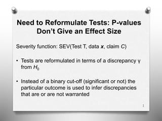
1. Need to Reformulate Tests: P-values
Don’t Give an Effect Size
Severity function: SEV(Test T, data x, claim C)
• Tests are reformulated in terms of a discrepancy γ
from H0
• Instead of a binary cut-off (significant or not) the
particular outcome is used to infer discrepancies
that are or are not warranted
1

2. An Example of SEV (3.2 SIST)
1-sided normal testing
H0: μ ≤ 150 vs. H1: μ > 150 (Let σ = 10, n = 100)
let significance level α = .025
Reject H0 whenever M ≥ 150 + 2σ/√n: M ≥ 152
M is the sample mean, its value is M0.
1SE = σ/√n = 1
2

3. Rejection rules:
Reject iff M > 150 + 2SE (N-P)
In terms of the P-value:
Reject iff P-value ≤ .025 (Fisher)
(P-value a distance measure, but inverted)
Let M = 152, so I reject H0.
3

4. PRACTICE WITH P-VALUES
Let M = 152
Z = (152 – 150)/1 = 2
The P-value is Pr(Z > 2) = .025
4

5. PRACTICE WITH P-VALUES
Let M = 151
Z = (151 – 150)/1 = 1
The P-value is Pr(Z > 1) = .16
(Note: SEV (μ > 150) = .84 = 1 – P-value for this test)
5

6. PRACTICE WITH P-VALUES
Let M = 150.5
Z = (150.5 – 150)/1 = .5
The P-value is Pr(Z > .5) = .3
6

7. PRACTICE WITH P-VALUES
Let M = 150
Z = (150 – 150)/1 = 0
The P-value is Pr(Z > 0) = .5
7

8. Frequentist Evidential Principle: FEV
FEV (i). x is evidence against H0 (i.e., evidence of
discrepancy from H0), if and only if the P-value Pr(d >
d0; H0) is very low (equivalently, Pr(d < d0; H0)= 1 - P
is very high).
8

9. Contraposing FEV(i) we get our minimal priniciple
FEV (ia) x are poor evidence against H0 (poor
evidence of discrepancy from H0), if there’s a high
probability the test would yield a more discordant
result, if H0 is correct.
Note the one-directional ‘if’ claim in FEV (1a)
(i) is not the only way x can be BENT.
9

10. H0: μ ≤ 150 vs. H1: μ > 150 (Let σ = 10, n = 100)
The usual test infers there’s an indication of some
positive discrepancy from 150 because
Pr(M < 152: H0) = .97
Not very informative
Are we warranted in inferring μ > 153 say?
10

11. • Recall the complaint of the Likelihoodist
(p. 36)
• For them, inferring H1: μ > 150 means
every value in the alternative is more likely
than 150
• Our inferences are not to point values, but
we block inferences to discrepancies
beyond those warranted with severity.
11

12. Consider: How severely has μ > 153 passed the test?
SEV(μ > 153 ) (p. 143)
M = 152, as before, claim C: μ > 153
The data “accord with C” but there needs to be a
reasonable probability of a worse fit with C, if C is false
Pr(“a worse fit”; C is false)
Pr(M ≤ 152; μ ≤ 153)
Evaluate at μ = 153, as the prob is greater for μ < 153.
12

13. Consider: How severely has μ > 153 passed the test?
To get Pr(M ≤ 152: μ = 153), standardize:
Z = √100 (152- 153)/10 = -1
Pr(Z < -1) = .16 Terrible evidence
13

14. Consider: How severely has μ > 150 passed the test?
To get Pr(M ≤ 152: μ = 150), standardize:
Z = √100 (152- 150)/1 = 2
Pr(Z < 2) = .97
Notice it’s 1 – P-value
14

15. Now consider SEV(μ > 150.5) (still with M = 152)
Pr (A worse fit with C; claim is false) = .93
Pr(M < 152; μ = 150.5)
Z = (152 – 150.5) /1 = 1.5
Pr (Z < 1.5)= .93 Fairly good indication μ > 150.5
15

16. 16
O Table 3.1
O Table 3.1

17. FOR PRACTICE:
Now consider SEV(μ > 151) (still with M = 152)
Pr (A worse fit with C; claim is false) = __
Pr(M < 152; μ = 151)
Z = (152 – 151) /1 = 1
Pr (Z < 1)= .84
17

18. MORE PRACTICE:
Now consider SEV(μ > 152) (still with M = 152)
Pr (A worse fit with C; claim is false) = __
Pr(M < 152; μ = 152)
Z = 0
Pr (Z < 0)= .5–important benchmark
Terrible evidence that μ > 152
Table 3.2 has exs with M = 153.
18

19. Using Severity to Avoid Fallacies:
Fallacy of Rejection: Large n
problem
• Fixing the P-value, increasing sample size n,
the cut-off gets smaller
• Get to a point where x is closer to the null than
various alternatives
• Many would lower the P-value requirement as n
increases-can always avoid inferring a
discrepancy beyond what’s warranted: 19

20. Severity tells us:
• an α-significant difference indicates less of a
discrepancy from the null if it results from larger (n1)
rather than a smaller (n2) sample size (n1 > n2 )
• What’s more indicative of a large effect (fire), a fire
alarm that goes off with burnt toast or one that
doesn’t go off unless the house is fully ablaze?
• [The larger sample size is like the one that goes off
with burnt toast] 20

21. (looks ahead) Compare n = 100 with n
= 10,000
H0: μ ≤ 150 vs. H1: μ > 150 (Let σ = 10, n = 10,000)
Reject H0 whenever M ≥ 2SE: M ≥ 150.2
M is the sample mean (significance level = .025)
1SE = σ/√n = 10/√10,000 = .1
Let M = 150.2, so I reject H0.
21

22. Comparing n = 100 with n = 10,000
Reject H0 whenever M ≥ 2SE: M ≥ 150.2
SEV10,000(μ > 150.5) = 0.001
Z = (150.2 – 150.5) /.1 = -.3/.1 = -3
P(Z < -3) = .001
Corresponding 95% CI: [0, 150.4]
A .025 result is terrible indication μ > 150.5
When reached with n = 10,000
While SEV100(μ > 150.5) = 0.93
22

23. Non-rejection. Let M = 151, the test does not reject H0.
The standard formulation of N-P (as well as Fisherian)
tests stops there.
We want to be alert to a fallacious interpretation of a
“negative” result: inferring there’s no positive
discrepancy from μ = 150.
Is there evidence of compliance? μ ≤ 150?
The data “accord with” H0, but what if the test had little
capacity to have alerted us to discrepancies from 150?
23

24. No evidence against H0 is not evidence for it.
Condition (S-2) requires us to consider Pr(X > 151;
150), which is only .16.
24

25. P-value “moderate”
FEV(ii): A moderate p value is evidence of the absence
of a discrepancy γ from H0, only if there is a high
probability the test would have given a worse fit with H0
(i.e., smaller P- value) were a discrepancy γ to exist.
For a Fisherian like Cox, a test’s power only has
relevance pre-data, they can measure “sensitivity”.
In the Neyman-Pearson theory of tests, the
sensitivity of a test is assessed by the notion of
power, defined as the probability of reaching a preset
level of significance …for various alternative
hypotheses. In the approach adopted here the
assessment is via the distribution of the random
variable P, again considered for various alternatives
(Cox 2006, p. 25)
25

26. Computation for SEV(T, M = 151, C: μ ≤ 150)
Z = (151 – 150)/1 = 1
Pr(Z > 1) = .16
SEV(C: μ ≤ 150) = low (.16).
• So there’s poor indication of H0
26

27. Can they say M = 151 is a good indication that μ ≤
150.5?
No, SEV(T, M = 151, C: μ ≤ 150.5) = ~.3.
[Z = 151 – 150.5 = .5]
But M = 151 is a good indication that μ ≤ 152
[Z = 151 – 152 = -1; Pr (Z > -1) = .84 ]
SEV(μ ≤ 152) = .84
It’s an even better indication μ ≤ 153 (Table 3.3, p. 145)
[Z = 151 – 153 = -2; Pr (Z > -2) = .97 ]
27

28. Π(γ): “sensitivity function”
Computing Π(γ) views the P-value as a statistic.
Π(γ) = Pr(P < pobs; µ0 + γ).
The alternative µ1 = µ0 + γ.
Given that P-value inverts the distance, it is less
confusing to write Π(γ)
Π(γ) = Pr(d > d0; µ0 + γ).
Compare to the power of a test:
POW(γ) = Pr(d > cα; µ0 + γ) the N-P cut-off cα.
28

29. FEV(ii) in terms of Π(γ)
P-value is modest (not small): Since the data accord
with the null hypothesis, FEV directs us to examine
the probability of observing a result more discordant
from H0 if µ = µ0 +γ:
If Π(γ) = Pr(d > d0; µ0 + γ) is very high, the data
indicate that µ< µ0 +γ.
Here Π(γ) gives the severity with which the test has
probed the discrepancy γ.
29

30. FEV (ia) in terms of Π(γ)
If Π(γ) = Pr(d > do; µ0 +γ) = moderately high (greater
than .3, .4, .5), then there’s poor grounds for
inferring µ > µ0 + γ.
This is equivalent to saying the SEV(µ > µ0 +γ) is
poor.
30

31. FEV/SEV (for Excur 3 Tour III)
Test T+: Normal testing: H0: µ < µ0 vs. H1: µ > µ0
σ known
(FEV/SEV): If d(x) is statistically significant (P- value
very small), then test T+ passes µ > M0 – k σ/√n with
severity (1 – ).
(FEV/SEV): If d(x) is not statistically significant (P- value
moderate), then test T+ passes µ < M0 + k σ/√n with
severity ( 1 – ),
where P(d(X) > k) = .
31