For any Assignment related queries, Call us at : - +1 678 648 4277
You can mail us at : - support@statisticsassignmenthelp.com or
reach us at : - https://www.statisticsassignmenthelp.com/
1. True or False (and state why).
(a). The significance level of a statistical test is not equal to the probability that the null hypothesis is
true.
Solution: True
(b). If a 99% confidence interval for a distribution parameter θ does not include θ0, the value under the
null hypothesis, then the corresponding test with significance level 1% would reject the null hypothesis.
Solution: True
(c). Increasing the size of the rejection region will lower the power of a test.
Solution: False
(d). The likelihood ratio of a simple null hypothesis to a simple alternate hypothesis is a statistic which
is higher the stronger the evidence of the data in favor of the null hypothesis.
Solution: True
(e). If the p-value is 0.02, then the corresponding test will reject the null at the 0.05 level.
Solution: True
2. Testing Goodness of Fit.
Let X be a binomial random variable with n trials and probability p of success.
(a). Suppose n = 100 and X = 38. Compute the Pearson chi-square statistic for testing the goodness of
fit to the multinomial distribution with two cells with H0 : p = p0 = 0.5.
(b). What is the approximate distribution of the test statistic in (a), under the null Hypothesis H0.
(c). What can you say about the P-value of the Pearson chi-square statistic in (a) using the following
table of percentiles for chi-square random variables ? (i.e., P(χ2 3 ≤ q.90 = 6.25) = .90 )
df q.90 q.95 q.975 q.99 q.995
1 2.71 3.84 5.02 6.63 9.14
2 4.61 5.99 7.38 9.21 11.98
3 6.25 7.81 9.35 11.34 14.32
4 7.78 9.49 11.14 13.28 16.42
(d). Consider the general case of the Pearson chi-square statistic in (a), where the outcome X = x is kept
as a variable (yet to be observed). Show that the Pearson chi-square statistic is an increasing function of
|x−n/2|.
(e). Suppose the rejection region of a test of H0 is {X : |X − n/2| > k} for some fixed known number k.
Using the central limit theorem (CLT) as an approximation to the distribution of X, write an expression
that approximates the significance level of the test for given k. (Your answer can use the cdf of Z ∼
N(0, 1) : Φ(z) = P(Z ≤ z).)
Solution:
(a). The Pearson chi-square statistic for a multinomial distribution with (m = 2) cells is
where the observed counts are
O1 = x = 38 and O2 = n − x = 62,
and the expected counts under the null hypothesis are
E1 = n × p0 = n × 1/2 = 50 and E2 = (n − x) × (1 − p0) = (n − x) × (1 − 1/2) = 50
Plugging these in gives
(b). The approximate distribution of X 2 is chi-squared with degrees of freedom q = dim({p, 0 ≤ p ≤
1}) − dim({p : p = 1/2}) = (m − 1) − 0 = 1.
(c). The P-value of the Pearson chi-square statistic is the probability that a chi-square random variable
with q = 1 degrees of freedom exceeds the 5.76, the observed value of the statistic. Since 5.76 is
greater than q.975 = 5.02 and less than q.99 = 6.63, (the percentiles of the chi-square distribution with
q = 1 degrees of freedom) we know that the P-value is smaller than (1 − .975) = .025 but larger than (1
− .99) = .01.
(d). Substituing O1 = x and O2 = (n − x) and E1 = n × p0 = n/2 and E2 = n × (1 − p0) = n/2 in the
formula from (a) we get
(e). Since X is the sum of n independent Bernoulli(p) random variables, E[X] = np and V ar(X) = np(1 −
p)
so by the CLT
X ∼ N(np, np(1 − p)) (approximately)
which is N( n , ) when the null hypothesis (p = 0.5) is true.
The significance level of the test is the probability of rejecting the null hypothesis when it is true which
is given by:
3. Reliability Analysis
Suppose that n = 10 items are sampled from a manufacturing process and S items are found to be
defective. A beta(a, b) prior 1 is used for the unknown proportion θ of defective items, where a > 0, and
b > 0 are known.
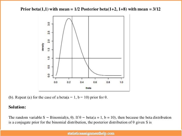
(a). Consider the case of a beta prior with a = 1 and b = 1. Sketch a plot of the prior density of θ and of
the posterior density of θ given S = 2. For each density, what is the distribution’s mean/expected value
and identify it on your plot.
Solution:
The random variable S ∼ Binomial(n, θ). If θ ∼ beta(a = 1, b = 1), then because the beta distribution is
a conjugate prior for the binomial distribution, the posterior distribution of θ given S is
beta(a∗ = a + S, b∗ = b + (n − s))
For S = 2, the posterior distribution of θ is thus beta(a = 3, b = 9)
Since the mean of a beta(a, b) distribution is a/(a + b), the prior mean is 1/2 = 1/(1 + 1), and the
posterior mean is 3/12 = (a + s)/(a + b + n)
These densities are graphed below
Prior beta(1,1) with mean = 1/2 Posterior beta(1+2, 1+8) with mean = 3/12
(b). Repeat (a) for the case of a beta(a = 1, b = 10) prior for θ.
Solution:
The random variable S ∼ Binomial(n, θ). If θ ∼ beta(a = 1, b = 10), then because the beta distribution
is a conjugate prior for the binomial distribution, the posterior distribution of θ given S is
beta(a∗ = a + S, b∗ = b + (n − s))
For S = 2, the posterior distribution of θ is thus beta(a = 3, b = 18)
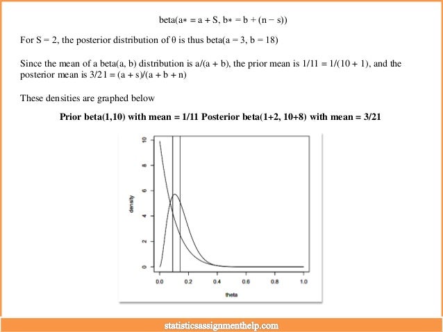
Since the mean of a beta(a, b) distribution is a/(a + b), the prior mean is 1/11 = 1/(10 + 1), and the
posterior mean is 3/21 = (a + s)/(a + b + n)
These densities are graphed below
Prior beta(1,10) with mean = 1/11 Posterior beta(1+2, 10+8) with mean = 3/21
(c). What prior beliefs are implied by each prior in (a) and (b); explain how they differ?
Solution:
The prior in (a) is a uniform distribution on the interval 0 < θ < 1. It is a flat prior and represents
ignorance about θ such that any two intervals of θ have the same probability if they have the same
width.
The prior in (b) gives higher density to values of θ closer to zero. The mean value of the prior in (b) is
1/11 which is much smaller than the mean value of the uniform prior in (a) which is 1/2.
(d). Suppose that X S = 1 or 0 according to whether an item is defective (X=1). For the general case of
a prior beta(a, b) distribution with fixed a and b, what is the marginal distribution of X before the n =
10 sample is taken and S is observed? (Hint: specify the joint distribution of X and θ first.)
Solution:
The joint distribution of X and θ has pdf/cdf:
f(x, θ) = f(x | θ)π(θ)
where f(x | θ) is the pmf of a Bernoulli(θ) random variable and π(θ) is the pdf of a beta(a, b)
distribution.
The marginal distribution of X has pdf
That is, X is Bernoulli(p) with p = θπ(θ)dθ = E[θ | prior] = a/(a+b).
(e). What is the marginal distribution of X after the sample is taken? (Hint: specify the joint
distribution of X and θ using the posterior distribution of θ.)
Solution:
The marginal distribution of X afer the sample is computed using the same argument as (c), replacing
the prior distribution with the posterior distribution for θ given S = s.
X is Bernoulli(p)
With
J 1 p = θπ(θ | S)dθ = E[θ | S] = (a + s)/(a + b + n).

Probability and Statistics Assignment Help

  • 1.
    For any Assignmentrelated queries, Call us at : - +1 678 648 4277 You can mail us at : - support@statisticsassignmenthelp.com or reach us at : - https://www.statisticsassignmenthelp.com/
  • 2.
    1. True orFalse (and state why). (a). The significance level of a statistical test is not equal to the probability that the null hypothesis is true. Solution: True (b). If a 99% confidence interval for a distribution parameter θ does not include θ0, the value under the null hypothesis, then the corresponding test with significance level 1% would reject the null hypothesis. Solution: True (c). Increasing the size of the rejection region will lower the power of a test. Solution: False (d). The likelihood ratio of a simple null hypothesis to a simple alternate hypothesis is a statistic which is higher the stronger the evidence of the data in favor of the null hypothesis. Solution: True (e). If the p-value is 0.02, then the corresponding test will reject the null at the 0.05 level. Solution: True
  • 3.
    2. Testing Goodnessof Fit. Let X be a binomial random variable with n trials and probability p of success. (a). Suppose n = 100 and X = 38. Compute the Pearson chi-square statistic for testing the goodness of fit to the multinomial distribution with two cells with H0 : p = p0 = 0.5. (b). What is the approximate distribution of the test statistic in (a), under the null Hypothesis H0. (c). What can you say about the P-value of the Pearson chi-square statistic in (a) using the following table of percentiles for chi-square random variables ? (i.e., P(χ2 3 ≤ q.90 = 6.25) = .90 ) df q.90 q.95 q.975 q.99 q.995 1 2.71 3.84 5.02 6.63 9.14 2 4.61 5.99 7.38 9.21 11.98 3 6.25 7.81 9.35 11.34 14.32 4 7.78 9.49 11.14 13.28 16.42 (d). Consider the general case of the Pearson chi-square statistic in (a), where the outcome X = x is kept as a variable (yet to be observed). Show that the Pearson chi-square statistic is an increasing function of |x−n/2|. (e). Suppose the rejection region of a test of H0 is {X : |X − n/2| > k} for some fixed known number k. Using the central limit theorem (CLT) as an approximation to the distribution of X, write an expression that approximates the significance level of the test for given k. (Your answer can use the cdf of Z ∼
  • 4.
    N(0, 1) :Φ(z) = P(Z ≤ z).) Solution: (a). The Pearson chi-square statistic for a multinomial distribution with (m = 2) cells is where the observed counts are O1 = x = 38 and O2 = n − x = 62, and the expected counts under the null hypothesis are E1 = n × p0 = n × 1/2 = 50 and E2 = (n − x) × (1 − p0) = (n − x) × (1 − 1/2) = 50 Plugging these in gives
  • 5.
    (b). The approximatedistribution of X 2 is chi-squared with degrees of freedom q = dim({p, 0 ≤ p ≤ 1}) − dim({p : p = 1/2}) = (m − 1) − 0 = 1. (c). The P-value of the Pearson chi-square statistic is the probability that a chi-square random variable with q = 1 degrees of freedom exceeds the 5.76, the observed value of the statistic. Since 5.76 is greater than q.975 = 5.02 and less than q.99 = 6.63, (the percentiles of the chi-square distribution with q = 1 degrees of freedom) we know that the P-value is smaller than (1 − .975) = .025 but larger than (1 − .99) = .01. (d). Substituing O1 = x and O2 = (n − x) and E1 = n × p0 = n/2 and E2 = n × (1 − p0) = n/2 in the formula from (a) we get (e). Since X is the sum of n independent Bernoulli(p) random variables, E[X] = np and V ar(X) = np(1 − p)
  • 6.
    so by theCLT X ∼ N(np, np(1 − p)) (approximately) which is N( n , ) when the null hypothesis (p = 0.5) is true. The significance level of the test is the probability of rejecting the null hypothesis when it is true which is given by: 3. Reliability Analysis Suppose that n = 10 items are sampled from a manufacturing process and S items are found to be defective. A beta(a, b) prior 1 is used for the unknown proportion θ of defective items, where a > 0, and b > 0 are known. (a). Consider the case of a beta prior with a = 1 and b = 1. Sketch a plot of the prior density of θ and of the posterior density of θ given S = 2. For each density, what is the distribution’s mean/expected value and identify it on your plot.
  • 7.
    Solution: The random variableS ∼ Binomial(n, θ). If θ ∼ beta(a = 1, b = 1), then because the beta distribution is a conjugate prior for the binomial distribution, the posterior distribution of θ given S is beta(a∗ = a + S, b∗ = b + (n − s)) For S = 2, the posterior distribution of θ is thus beta(a = 3, b = 9) Since the mean of a beta(a, b) distribution is a/(a + b), the prior mean is 1/2 = 1/(1 + 1), and the posterior mean is 3/12 = (a + s)/(a + b + n) These densities are graphed below
  • 8.
    Prior beta(1,1) withmean = 1/2 Posterior beta(1+2, 1+8) with mean = 3/12 (b). Repeat (a) for the case of a beta(a = 1, b = 10) prior for θ. Solution: The random variable S ∼ Binomial(n, θ). If θ ∼ beta(a = 1, b = 10), then because the beta distribution is a conjugate prior for the binomial distribution, the posterior distribution of θ given S is
  • 9.
    beta(a∗ = a+ S, b∗ = b + (n − s)) For S = 2, the posterior distribution of θ is thus beta(a = 3, b = 18) Since the mean of a beta(a, b) distribution is a/(a + b), the prior mean is 1/11 = 1/(10 + 1), and the posterior mean is 3/21 = (a + s)/(a + b + n) These densities are graphed below Prior beta(1,10) with mean = 1/11 Posterior beta(1+2, 10+8) with mean = 3/21
  • 10.
    (c). What priorbeliefs are implied by each prior in (a) and (b); explain how they differ? Solution: The prior in (a) is a uniform distribution on the interval 0 < θ < 1. It is a flat prior and represents ignorance about θ such that any two intervals of θ have the same probability if they have the same width. The prior in (b) gives higher density to values of θ closer to zero. The mean value of the prior in (b) is 1/11 which is much smaller than the mean value of the uniform prior in (a) which is 1/2. (d). Suppose that X S = 1 or 0 according to whether an item is defective (X=1). For the general case of a prior beta(a, b) distribution with fixed a and b, what is the marginal distribution of X before the n = 10 sample is taken and S is observed? (Hint: specify the joint distribution of X and θ first.) Solution: The joint distribution of X and θ has pdf/cdf: f(x, θ) = f(x | θ)π(θ) where f(x | θ) is the pmf of a Bernoulli(θ) random variable and π(θ) is the pdf of a beta(a, b) distribution. The marginal distribution of X has pdf
  • 11.
    That is, Xis Bernoulli(p) with p = θπ(θ)dθ = E[θ | prior] = a/(a+b). (e). What is the marginal distribution of X after the sample is taken? (Hint: specify the joint distribution of X and θ using the posterior distribution of θ.) Solution: The marginal distribution of X afer the sample is computed using the same argument as (c), replacing the prior distribution with the posterior distribution for θ given S = s. X is Bernoulli(p) With J 1 p = θπ(θ | S)dθ = E[θ | S] = (a + s)/(a + b + n).