Towards reducing the

International Journal of Data Mining & Knowledge Management Process (IJDKP) Vol.6, No.1, January 2016
DOI : 10.5121/ijdkp.2016.6103 27
TOWARDS REDUCING THE
MULTIDIMENSIONALITY OF OLAP CUBES
USING THE EVOLUTIONARY ALGORITHMS
AND FACTOR ANALYSIS METHODS
Sami NAOUALI and Semeh BEN SALEM
Virtual Reality and Information Technologies LAB,
Military Academy of Fondouk Jedid, TUNISA
snaouali@gmail.com
Semeh.bensalem@yahoo.fr
ABSTRACT
Data Warehouses are structures with large amount of data collected from heterogeneous sources to be
used in a decision support system. Data Warehouses analysis identifies hidden patterns initially unexpected
which analysis requires great memory and computation cost. Data reduction methods were proposed to
make this analysis easier. In this paper, we present a hybrid approach based on Genetic Algorithms (GA)
as Evolutionary Algorithms and the Multiple Correspondence Analysis (MCA) as Analysis Factor Methods
to conduct this reduction. Our approach identifies reduced subset of dimensions p’ from the initial subset p
where p'<p where it is proposed to find the profile fact that is the closest to reference. Gas identify the
possible subsets and the Khi² formula of the ACM evaluates the quality of each subset. The study is based
on a distance measurement between the reference and n facts profile extracted from the warehouse.
KEYWORDS
Data Warehouse, OLAP cube, dimensions reduction, Genetic Algorithms, Multiple Correspondence
Analysis
1. INTRODUCTION
Data Warehouses (DW) are used to collect and store great data quantity in large tables to be then
processed which helps extracting knowledge and assist in decision making. DW collects the data
stored from heterogeneous sources and creates centralized huge data bases to identify initially
hidden patterns once treated. In (W. INMON, 1994), the authors present these large data
structures and their architecture as a result of the data gathering from centralized relational
databases initially decentralized which can homogenize them and offer the possibility to treat and
process them which is initially a hard task. Graphically, these data sets can be represented by
cubic multidimensional data structures called OLAP cubes. (L.Lebart, A.Morineau, M.Piron,
2006) consider the multidimensional statics as an interesting analysis axis that should be studied.
The random assembly of data and their arrangement in the DW may contain unnecessary and
superfluous data that have no real interest for the analyst and can even provide incorrect results if

28
included in the processing. To facilitate the exploitation and interpretation of the DW, it is
necessary to propose innovative methods in order to reduce the huge amount of data contained in
the DW. The reduction methods proposed focuses mainly on reducing either the lines or the
columns of the DW.
In this context, we propose in this paper an approach based on the use of two methods: Genetic
Algorithms (GAs) and the Multiple Correspondence Analysis (MCA). The combination of these
two methods makes it possible to converge, using a specified process, to an optimum solution in
a set of possible ones. This new solution that has been identified helps identifying the most
appropriate dimensions that can be reduced and determining the best subset of dimensions that
best summarizes the DW.
In this paper, the second section details the previous work in relation with the topic of reduction
and exposes their limitations. The third section presents the two techniques we suggest to use in
our approach. The third section explains the approach and the adaptation of the tools used to the
multidimensional context, an algorithm representing the whole process is also presented in this
section. In section four, we present an illustrative example and we finish by interpreting the
results and giving our conclusion and perspectives.
2. RELATED WORKS AND MOTIVAIONS
The objective of reducing the data in a DW is to provide greater clarity of the information stored
and facilitates their processing which keeps only the information with a real interest. In this
context, several proposals were made, either by removing data stored for a long period of time,
aggregating them or reduce the dimensions and facts. Each of these approaches has its limits we
propose to identify in the following paragraph.
In (S.Naouali, 2012), the author proposes a hybrid approach to reduce the dimensions of a DW by
applying the Rough Sets Theory (RST)(Pawlak, 1995) and the Principal Component Analysis
(PCA) (I. Jolliffe, 2002). The RST identifies and removes redundant and needless facts while the
PCA is used for quantitative data tables to reduce the number of dimensions. However, the
reduction represents in its self a loss of information seeing that some dimensions will be ignored.
On the other hand, this approach concerns only great quantitative data tables.
In (J. Skyt, C.S. Jensen, T.B. Pedersen, 2001),the authors propose to proceed by aggregating the
data to move to a higher level of granularity of the DW dimensions. This technique can lead to
the loss or non-visibility of some details which is binding for the analyst. The use of aggregation
functions allows passing from a granularity level to another. Such a methodology can hide certain
details with big importance for the analyst and as a result can bring confusion.
(C. S. Jensen, 1995) proposes to remove the historical data that has exceeded a certain limit,
considering that such information is no longer useful given the time elapsed which can be critical
because the deleted data may contain useful information and can power a recent model using old
stored data.
(W.Wang, J.Feng, H.Lu, J.Xu Yu, 2002) propose an approach towards reducing the lines (facts)
of a cube by creating a condensed cube with a smaller size than the non condensed one which

29
would help reduce its computation time.The approach explores the properties of single tuples so
that a number of tuples in a cube can be condensed into one without loss of any information.
In our approach, we propose to use one of the methods of factor analysis, the MCA associated
with the theory of Genetic Algorithms and consider the problem as an approximation approach:
we identify first the possible subsets in concordance with the problematic and then evaluate the
quality of each solution to either retain it or remove it.
3. REQUIRED PRIOR KNOWLEDGE AND TECHNIQUES
3.1 Evolutionary Algorithms
Evolutionary algorithms are stochastic algorithms inspired from the theory of evolution of
species, and used to solve optimization problems. They define a set of possible solutions
evaluated to converge to the best results. Three major families of algorithms have been proposed
as evolutionary algorithms:
The evolutionary strategies (H.-G. Beyer, H.-P. Schwefel,2002), to solve continuous optimization
problems.
Evolutionary Programming, considered as a method of artificial intelligence to the finite state
automata design.
Genetic algorithms (D. Goldberg, 1994).
In our approach, we use the GAs as optimization algorithms which process helps identifying the
most optimal solution to a specified problem. Each individual is represented by a chromosome
that represents a potential solution and must meet the constraints of the problem enunciated. The
initial population contains N individuals randomly coded. A fitness function will be used to
evaluate the quality of each solution contained in a population. A selection operator (J .Baker,
1995) will be then applied to keep individuals who were considered sufficiently relevant and can
give birth to more optimal solutions. The most optimal solutions obtained will be then included in
the next generation i+1 using the selection operator. The multiplication of the individuals is the
same generation is executed with the crossover operator and the mutation operator.
3.2 Factor Analysis Method
Factor analysis is a descriptive method used to describe a set of observed variables by latent ones
(not observed). This method of analysis helps reducing the data amount in great data tables by
reducing the number of variables. Each factorial method is associated to a particular type of data.
The most known factor analysis methods are:
The Principal Component Analysis (PCA) for quantitative variables.
The Multiple Correspondence Analysis (MCA) for qualitative variables.
Mixed Data Factor Analysis (MDFA) for mixed tables.
The Multiple Factor Analysis (MFA) for mixed tables grouped data.
The Hierarchical Multiple Factor Analysis (HMFA) to generalize the AFM.
The Factor Analysis of Correspondences (FAC) is dedicated to contingency tables.

30
In our approach, we propose to use, in the process of the GAs, a fitness function extracted from
the MCA. The choice of the fitness fitness is very important in this study. It should meet the
constraint of the approach to avoid producing mistaken results. The fitness fucntion we propose
to exploit corresponds to the Khi² formula used to compute the similarity between two
individuals by measuring the distance betwwen their respective caracteristics. The MCA is used
for large qualitative data tables. A data table with I individuals and J variables is then represented
by a matrix with I rows and J columns, xij represents the modality of the variable j possessed by
the individual i. In (J.Pagès, F.Husson, 2009), the authors present special tables of the MCA:
Table of Condensed Coding (TCC), specified by the user and submitted to the processing
software for analysis. The Complete Disjunctive Table (CDT) that contains in lines the
individuals as presented in the TCC, and in columns the different modalities. If kjis the number of
modalities of the variable j, the total number of modalities is then K = ∑ kjj . The number of
individuals in the rows corresponds to the same number as in the CDT. The total number of
modality is K୨ and we have:
൜
݇௜௝ = 1 ݂݅ ݅݊݀݅‫݈ܽݑ݀݅ݒ‬ ܿ‫ݏ݊݅ܽݐ݊݋‬ ݉‫ݕݐ݈݅ܽ݀݋‬ ݆
݇௜௝ = 0 ݈݁‫݁ݏ‬
ൠ
Table 1.Matrix of the TCC table data.
TCC =
1 Λ
j Λ
P
1 Μ
Μ Μ
i Λ Λ ijx
Λ Λ
Μ Μ
n Μ
Table2: Matrix of the CDT table data.
CDT=
1 Λ
J Λ
݇௝
1 Μ
Μ Μ
i Λ Λ ijk
Λ Λ
Μ Μ
n Μ
In our approach the formula which will be used to enable this evaluation corresponds to the Khi²
formula and is given by:
݀ଶሺ‫,ݏ‬ ‫′ݏ‬ሻ = ෍
1
݂௜.
൬
݇௜௦
݊௦
−
݇௜௦′
݊௦′
൰ ² = ݊ ෍ ൬
݊௜௦
݊௦
−
݊௜௦′
݊௦′
൰ ²
௡
௜ୀଵ
௡
௜ୀଵ
4. PROPOSED APPROACH FOR DATA WAREHOUSE REDUCTION
In our approach, we propose a method to reduce the number of dimensions p of a DW using the
AGs and the MCA. We try to identify a subset p’ of dimensions where p'<p, in which we can find
the closest elements to the reference. Each individual returned by the GA represents a subset of
dimensions and is considered as a possible solution. Every solution is represented by a
chromosome containing as many genes as the DW dimensions. Each gene has two possible
values: 1 if we keep the corresponding dimension in the solution and 0 otherwise. We then
calculate for each solution, the distance between the reference and each fact contained in the
extracted sample from the DW. We then consider the minimum value of the distances computed:
if we choose to make the sum of all the distances computed we wouldn’t be able to identify the

31
facts with minimum values and that are close to the reference. The approach is based on the
measure of similarity between two individuals.
The profile of interesting facts can then be ignored. Selecting the minimum in each step of the
calculation helps identifying the facts that are the closest to the reference according to the
distances measured with associated reductions. We have then two results at the same time: closest
elements to the reference in the sample and associated reduction. In all cases, the lower the
distance is, the most appropriate is the subset. The fitness function used to evaluate the quality of
the individuals is the Khi² formula deduced from the MCA and presented above. This formula,
applied to the multidimensional concept then becomes as follows :
݀ଶሺ݅, ݅′ሻ =
1
‫݌‬
෍
ሺ‫ݔ‬௜ − ‫ݔ‬௜ᇱሻ²
݉
݊⁄
ఈ
ఓୀଵ
=
݊
‫݌‬
෍
ሺ‫ݔ‬௜ − ‫ݔ‬௜ᇱሻ²
݉
ఈ
ఓୀଵ
p represents the number of dimensions of the DW, n the number of elements in the sample, µ a
modality or member of a dimension, m number of occurrence of µ ,α number of modalities in
dimensions. If the number of occurrences m increases the modality is more frequent in the
population.
The different steps of calculation and processing data are as follows:
1. Creating ܲ௜௡௜௧ of N individuals by the process of GAs corresponding to the first
generation.
2. Selecting a sample of N’ elements from the DW to use for the calculation of distances.
3. Creation of the TCC table.
4. Creation of the CDT table.
5. Calculation of the distances.
6. Generation of the next generation with the operators cross over and mutation.
The algorithm corresponding to such a process is given by:
FUNCTION GEN_ࡼ (N, P)
1. for each ݅݊݀௜,ଵஸ௜ஸே do
2. for each ݃݁݊݁௝,ଵஸ௝ஸ௉ do
3. ݅݊݀௜ൣ݃݁݊݁௝൧ ← rondom(1,0)
4. end for
5. end for
END GEN_ࡼ࢏࢔࢏࢚
FUNCTION GEN_TCC (P, α)
6. for each ݂ܽܿ‫ݐ‬௜,ଵஸ௜ஸே′ do
7. ܾܶܽ௜,௝;ଵஸ௜ஸே′;ଵஸ௝ஸ௉ ← ݂ܽܿ‫ݐ‬௜,௝;ଵஸ௜ஸே′;ଵஸ௝ஸ௉
8. end for

32
9. for each ܶ‫ܤܣ‬௜,௝;ଵஸ௜ஸே′;ଵஸ௝ஸ௉ do
10. ܶ‫ܥܥ‬ே′,௉ ← ܿ‫݃݊݅݀݋‬ ଴,ଵሺܶ‫ܤܣ‬௜,௝, ࢻ, ܲሻ
11. end for
END GEN_TCC
FUNCTION GEN_TDC (P, α)
12. for each ܶ‫ܥܥ‬ே′,௉ do
13. ܶ‫ܥܦ‬ே′,ௗ௜௠ ← ܿ‫݃݊݅݀݋‬ ଴,ଵሺܶ‫ܥܥ‬ே′,௉, ࢻ, ܲሻ (dim is the total number of dimension)
14. end for
END GEN_TDC
FUNCTION COMPUTE (N, α)
15. occ ← 0
16. som ← 0
17. for each ܶ‫ܥܦ‬௜,௝;ଵஸ௜ஸே′,ଵஸ௝ஸௗ௜௠ do
18. if ܶ‫ܥܦ‬௜,௝ = 1 then occ ← occ+1
19. end if
20. end for
21. for each ݅݊݀௜ൣ݃݁݊݁௝൧
22. if ݅݊݀௜ൣ݃݁݊݁௝൧ = 1 then
23. for each ܶ‫ܥܦ‬௞,௟;ଵஸ௞ஸே′,ଵஸ௟ஸௗ௜௠ do
24. A= math.pow((ܶ‫ܥܦ‬௞,௟- ref)),2)/occ
25. som ← som+A
26. end for
27. else
28. for each ܶ‫ܥܦ‬௞,௟;ଵஸ௞ஸே′,ଵஸ௟ஸௗ௜௠{௝} do
29. A= math.pow((ܶ‫ܥܦ‬௞,௟- ref)),2)/occ
30. som ← som+A
31. dist[] ← min ሺ‫݉݋ݏ‬ሻ
32. end for
END COMPUTE
Selection operator, we only keep distances computed and corresponding to individuals that are
lower than a certain limit
FUNCTION SELECTION (N, limit)
33. for each ݅݊݀௜ൣ݃݁݊݁௝൧ ∈ ‫ܩ‬௜ do
34. if ݅݊݀௜ሺ݀݅‫ݐݏ‬ሻ < limit
35. then ݅݊݀௜ൣ݃݁݊݁௝൧ ∈ ‫ܩ‬௜ାଵ

33
36. end if
37. end for
END SELECTION
Crossing of two individuals to generate two children (crossover operator)
FUNCTION CROSSOVER ()
38. cross_pos ← random(1,2,3,4,5)
39. aux[k ← 0]
40. for each ݅݊݀௜ൣ݃݁݊݁௝൧ do
41. for each ݅݊݀௜ൣ݃݁݊݁௖௥௢௦௦_௣௢௦൧ do
42. aux[][k]← ݅݊݀௜ൣ݃݁݊݁௝൧
43. ݅݊݀௜ൣ݃݁݊݁௝൧ ← ݅݊݀௜ାଵൣ݃݁݊݁௝൧
44. ݅݊݀௜ൣ݃݁݊݁௝൧ ← aux[k][]
45. end for
46. end for
END CROSSOVER
/* Mutation of two children with a probabilityp୫ (mutation operator) */
FUNCTION MUTATION ()
47. mut_pos ← random(1,2,3,4,5,6)
48. nb_mut ∈ {1,2,3,4,5,6}
49. for k from 1 to nb_mut do
50. for each ݅݊݀௜ൣ݃݁݊݁௝൧ do
51. if ݅݊݀௜ൣ݃݁݊݁௠௨௧_௣௢௦൧ ==0 then ݅݊݀௜ൣ݃݁݊݁௠௨௧_௣௢௦൧ ← 1 else ݅݊݀௜ൣ݃݁݊݁௠௨௧_௣௢௦൧ ← 0
52. end if
53. end for
54. end for
END MUTATION
5. APPLICATION ON AN EXAMPLE
In this section, it is proposed to apply the approach and the algorithm presented in section 4 on
the example of DW shown in Figure1. The objective of the DW is to collect information on
travellers at the border state offices posts to constitute a Big Data tables to learn about their
movements and monitor their traffic. The DW is formed by six DIMENSIONS TABLES and a
central FACTS TABLE.

34
Figure 1: Fact table and dimensions of the DW.
The different dimensions are {TRAVELLER, PASSEPORT, TRAVEL, DESTINATION,
CONTACT, BORDER CONTROL}. The DW contains qualitative data where each dimension
has a limited and fixed number of possible values presented as follows:
TRAVELLER{ Foreign, Citizen}
PASSEPORT{ Normal, Diplomatic, Mission }
TRAVEL{ Leisure, Professional }
DESTINATION{Asia, Africa, Western Europe, South America, Australia, North America,
Eastern Europe }
CONTACT{Person, Company}
BORDER CONTROL{Aerial, Earth, Maritime}
As we have explained in section 3.2, two special structures are considered in the MCA theory
during the process of calculation: the TCC and the CDT. In the following paragraph, we present
these two structures and their proposed adaptation to our example.
The MCA is used to measure the quality of the solutions returned by the process of GAs by
applying the Khi² formula. We consider a sample of N’ facts extracted from the DW since the
Khi² formula contains the parameter m representing the occurrence number of each modality in
the sample. The TCC represents the initial values taken by the dimensions of that sample but in
binary notation. The following Table 3 presents the sample with discrete values we propose to
consider:

35
Table 3: Extracted sample of facts from the DW
DIM1
TRAVELLER
DIM2
PASSEPORT
DIM3
TRAVEL
DIM4
DESTINATION
DIM5
CONTACT
DIM6
BORDER
CONTROL
IND1 Foreign Normal Leisure Asia Person Aerial
IND2 Citizen Diplomatic Leisure Africa Company Earth
IND3 Citizen Mission Professional Western Europe Person Maritime
IND4 Foreign Diplomatic Professional South America Person Maritime
IND5 Citizen Mission Leisure Asia Company Maritime
IND6 Foreign Normal Professional Africa Person Earth
IND7 Citizen Diplomatic Leisure Australia Company Aerial
IND8 Foreign Normal Leisure South America Person Maritime
IND9 Foreign Diplomatic Professional North America Company Earth
IND10 Citizen Mission Professional Eastern Europe Person Earth
For each sample extracted, a TCC, corresponding to the dimensions of the DW, will be generated
and will represent the same information initially stored in the data warehouse but encoded in
binary notation. Each value taken by the fact in the corresponding dimension will be encoded in a
binary notation. The corresponding TCC to the sample then considered is given by the following
Table 4:
Table 4: TCC corresponding to the extracted sample.
DIM1 DIM2 DIM3 DIM4 DIM5 DIM6
IND1 01 010 01 000001 10 001
IND2 10 001 10 001000 01 010
IND3 10 100 10 010000 10 100
IND4 01 001 10 100000 10 100
IND5 10 100 01 000001 01 100
IND6 01 010 10 001000 10 010
IND7 10 001 01 000010 01 001
IND8 01 010 01 100000 10 100
IND9 01 001 10 010000 01 010
IND10 10 100 10 001000 10 010
The second structure presented in the MCA theory concerns the CDT that represents the whole
modalities of the DW and not only the dimensions. The TCC represents a collection of binary
values, 0 or 1 arranged according to the dimensions of the DW. This table couldn’t then give an
understandable idea about the different modalities of the DW. Consequently, the CDT will be
used to give a more detailed view of the data in the DW according to the modalities considered.
This table will be used the Khi² formula during the calculation process. It also helps identifying
some necessary parameters for the computation such as the parameter m representing the number
of occurrences of each modality. The corresponding CDT to the sample considered previously is
presented by the following Table5:

36
Table 5: CDT corresponding to the extracted sample.
dim1 dim2 dim3 dim4 dim5 dim6
Mod1
Mod2
Mod1
Mod2
Mod3
Mod1
Mod2
Mod1
Mod2
Mod3
Mod4
Mod5
Mod6
Mod7
Mod1
Mod2
Mod1
Mod2
Mod3
CDT=
0 1 0 1 0 0 1 0 0 0 0 0 0 1 1 0 0 0 1 IND1
0 1 0 0 1 0 1 0 0 1 0 0 0 0 0 1 0 1 0 IND2
1 0 0 1 0 1 0 0 1 0 0 0 0 0 0 1 1 0 0 IND3
0 1 1 0 0 1 0 1 0 0 0 0 0 0 1 0 1 0 0 IND4
0 1 0 0 1 0 1 0 0 0 0 1 0 0 0 1 1 0 0 IND5
1 0 0 1 0 1 0 0 0 0 1 0 0 0 0 1 0 1 0 IND6
0 1 1 0 0 0 1 0 0 0 0 0 1 0 1 0 0 0 1 IND7
1 0 0 1 0 0 1 0 0 0 0 0 1 0 1 0 1 0 0 IND8
0 1 1 0 0 1 0 0 1 0 0 0 0 0 1 0 0 1 0 IND9
0 1 0 0 1 1 0 0 0 1 0 0 0 0 0 1 0 1 0 IND10
ref 1 0 0 1 0 0 1 0 0 0 1 0 0 0 0 1 0 0 1
The CDT and the TCC obtained transform the discrete qualitative data into a binary set of data
which facilitates their calculation using the Khi² adapted formula. This formula is used to
measure the degree of similarity between individuals. Each individual will have an encoding of
19-bit representing its whole characteristic profile. The encoding of the individuals in this table is
not aleatory; it should respect the following findings to preserve the integrity of the table: the
number of bits encoded 1 in a line is equal to P (number of dimensions) and the number of
occurrences m for each dimension is equal to N’ (number of elements in the sample)
In the process of GAs, each solution will be encoded by a 6 bits chromosome which corresponds
to the number of dimensions. Each gene is coded 1 if the corresponding dimension exists for the
individual and 0 otherwise. The total number of possible solutions is then26
= 64.
6. RESULTS INTERPRETATION
As already defined, the purpose of the study is to reduce the DW dimensions by determining the
most suitable subset of dimensions where the sample of facts retained contains the closest to the
reference. For this, it is proposed to measure the distance between the reference profile refx
and
all the other individuals xi of the selected sample taking into consideration the reduced
dimensions. We will then try to identify the elements in the sample which profile is similar to the
reference profile.
In the calculation process, it is considered to compute ten values of distances. It is then proposed
to retain the minimum one as the distance between the reference and that element. If we sum all
the measures, we couldn’t then identify the closest individuals to the reference since they will be
hidden by the sum. For each step of computation, we should take into consideration the solutions
returned by the process of the GAs.
This calculation could be performed in two ways: the first one is to compute the distances and
keep in the CDT the dimensions retained by the GA and replace all the rest of the values by 0.
The second one consists on totally removing the not retained dimensions in the GAs proposal and

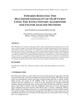
37
excluding them from the calculation as well as the reference. We then consider the minimum
value among all the measures.
An illustrative example is given as follows: The solution returned by the process of the GA is:
011010 where we choose to keep the subset of dimensions (235). The distances were measured
between the reference given in the CDT and each element of the sample considered. We then
obtain the results presented in the Table 6 below:
Table 6: Results corresponding to the reduction.
INDIVIDUALS ‫ݔ‬௥௘௙, ‫ݔ‬ଵ ‫ݔ‬௥௘௙, ‫ݔ‬ଶ ‫ݔ‬௥௘௙, ‫ݔ‬ଷ ‫ݔ‬௥௘௙, ‫ݔ‬ସ ‫ݔ‬௥௘௙, ‫ݔ‬ହ ‫ݔ‬௥௘௙, ‫ݔ‬଺ ‫ݔ‬௥௘௙, ‫ݔ‬଻ ‫ݔ‬௥௘௙, ‫ݔ‬଼ ‫ݔ‬௥௘௙, ‫ݔ‬ଽ ‫ݔ‬௥௘௙, ‫ݔ‬ଵ଴
‫ܦ‬௄௛௜
ଶ
(‫ݔ‬௥௘௙, ‫ݔ‬௜) 3,573 3,867 3,573 5,147 3,867 3,573 4,507 3,573 5,147 4,507
The minimum distances were obtained for individualsxଵ, xଷ, x଺ and x଼ which explains that with
the reduction (235), we first detect 4 minimum values which mean that the sample of ten
elements considered contains four individuals that are the closest to the reference with an average
of 40%. The value that will be retained in the processing is D୏୦୧
ଶ
= 3.57 as the minimum value of
distance corresponding to this reduction.
The same previous reasoning was also applied for all the other reductions, retaining for each time
the minimum value computed. We then obtain the following Figure 2:
Figure 2: Distance measurement with reference with reduction
According to the previous curve, for each number of retained dimensions, we identify two
subsets: one for minimum distances and the other for maximum ones, which means that for each
group of solutions we can identify maximum and minimum measures. In our approach it is
proposed to conserve only groups corresponding to the minimum results to get closer as much as
possible to the reference. Providing the analyst with these results can assist him in choosing the
right reduction configuration.
Distance computation is mainly used for segmentation process to identify similar groups
containing individuals with similar characteristics. Our approach is based on a measure of
similarity between a reference and all the individuals of the sample considered. We can by the
way change the configuration of the reference whenever the analyst wishes.

38
7. CONCLUSIONS AND PERSPECTIVES
Collecting and storing information in a DW creates huge data structures which analysis is a
complex task. These DW could be visualized in multidimensional structures called OLAP cubes
according to multiple analysis axes. To make the analysis process of the DW easier, data
reduction methods have been proposed where the reduction may concern either the number of
facts (lines) or dimensions (columns) of the warehouse. Our approach is based on the use of GAs
and the MCA, to express the similarity between a reference and a group of individuals to find the
most similar individual in the sample to the reference by using the Khi² formula. The method
provided is used only for qualitative data which is a great limitation because analysis can also
concern quantitative data. The process identifies groups of distances corresponding to different
distances some are maximum and others are minimum. The analyst can then choose which
solution fits the requirements of the analysis. In all cases, the reduction corresponds to a loss of
information either by replacing the values by 0 for the not retained dimensions or by eliminating
them from the computation. In our case, we have applied a technique based on distances
measurement widely used for segmentation and clustering to identify the most appropriate
dimensions reductions in a DW.
REFERENCES
[1] W. H. INMON. (1994). Builiding the Data Wharehouse Toolkit. Wiley Computer Publishing, ISBN 0-471-
56960-7
[2] L.Lebart, A.Morineau, M.Piron (2006). Statistique exploratoire multidimensionnelle. Dunod, Paris
[3] Sami Naouali. (2012) “Hybrid Approach Toward Reducing Data Cubes”, DAWAK’2012, Copenhagen,
Denmark.
[4] Z. Pawlak, J. Grzymala-Busse, R. Slowinski, W. Ziarko. (1995). Rough Sets, Common ACM 38, pp 88-95.
[5] I. Jolliffe (2002). Principal Component Analysis,Springer-Verlag.
[6] J. Skyt, C.S. Jensen, T.B. Pedersen. (2001). Specified-based Data Reduction in Dimensional Data
Warehouses. TimeCenter TechReport TR-61.
[7] C. S. Jensen. (1995) “Vacuuming”, in the TSQL2 Temporal Query Language, R. T. Snodgrass editor,
Chapter 23, pp. 451-462, Kluwer Academic Publishers.
[8] Wei Wang, Jianlin Feng, Hongjun Lu, Jeffrey Xu Yu. (2002) “ Condensed Cube: An Effective Approach
to Reducing Data Cube Size”, Proceedings of the 18th International Conference on Data Engineering
(ICDE)
[9] H.-G. Beyer et H.-P. (2002) Schwefel, Evolution Strategies: A Comprehensive Introduction, Natural
Computing, volume 1, numéro 1, pages 3-52.
[10] D. Goldberg. (1994), Algorithmes génétiques, Addison–Wesley France.
[11] James Edward Baker, Adaptive Selection Methods for Genetic Algorithms, Computer Science
Departement, Vanderbilt University
[12] Jérôme Pagès, “Analyse des Correspondances Multiples ACM, introduction à l’aide d’un exemple”
Laboratoire de mathématiques appliqués Agrocampus, Rennes.

Towards reducing the

Recommended

Recommended

More Related Content

What's hot

What's hot (20)

Viewers also liked

Viewers also liked (20)

Similar to Towards reducing the

Similar to Towards reducing the (20)

Recently uploaded

Recently uploaded (20)

Towards reducing the