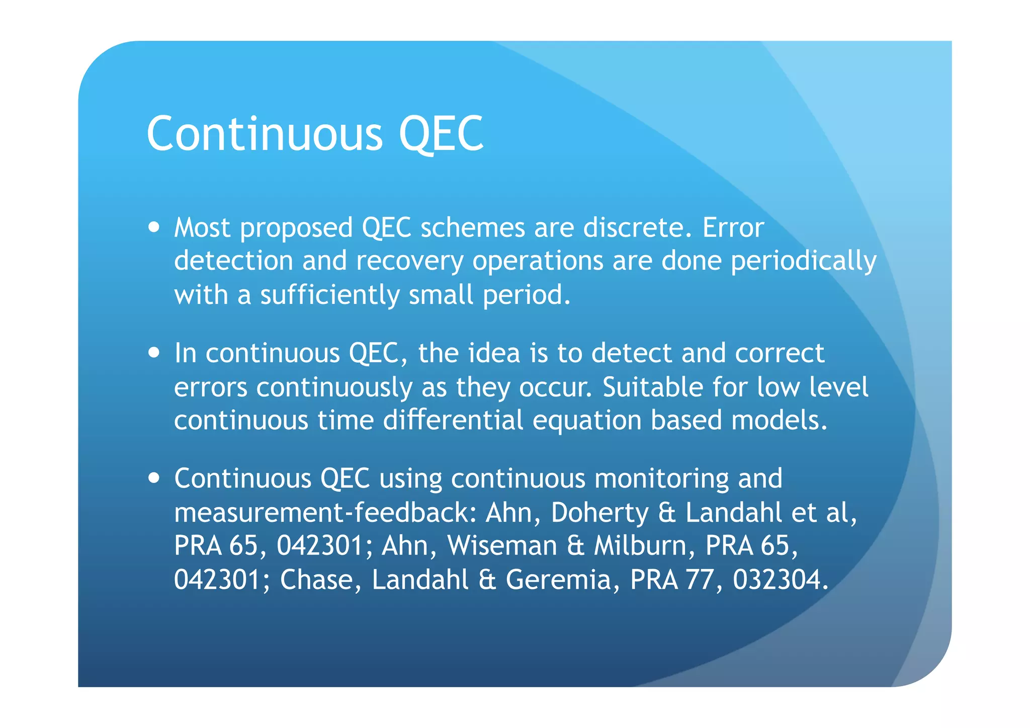
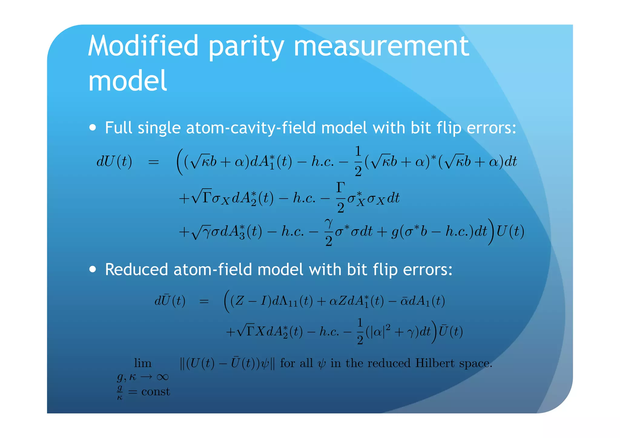
The document presents a coherent-feedback formulation for a continuous quantum error correction (QEC) protocol, focusing on a simple 3 qubit bit flip code. It outlines the principles of quantum error correction, continuous monitoring, and the advantages of coherent-feedback systems over traditional discrete QEC schemes. The study emphasizes on-chip implementations and describes how coherent lasers can facilitate corrections in a quantum computing context.

1. Coherent-Feedback Formulation
of a Continuous Quantum Error
Correction Protocol
arXiv:0907.0236
Hendra Nurdin
(The Australian National University)
Joint work with:
Joe Kerckhoff
Dmitri Pavlichin
Hideo Mabuchi
(Stanford University)

2. Talk plan
 Reminder of quantum error correction (QEC).
 Continuous QEC.
 Description of a scheme for coherent-feedback QEC for
a simple 3 qubit bit flip code.
 Concluding remarks.

3. Quantum error correction (QEC)
 Quantum error correction is essential for quantum
information processing since qubits are susceptible to
decoherence.
 When decoherence alters the state of a qubit, a QEC
algorithm acts to restore it to the state prior to
decoherence.

4. QEC principles
 Main ingredient is to introduce reduncancy by encoding
a logical qubit into a number of physical qubits.
 Simple 3 qubit code: A logical qubit is encoded by 3
physical qubits. Logical qubit |0 >L encoded by 3
physical qubits |000 > and |1 >L encoded by |111 >.
 A logical state a|0 >L + b|1 >L is encoded as a|000 > + b|
111 >. The 3 qubit codespace is C = span{|000 >,|111>}.

5. The 3 qubit bit flip code
 This simple code belongs to a class of QEC codes called
stabilizer codes (Gottesman, PRA 54, 1862)
 C = span{| 000 >,|111 >}
 Correctable errors are single qubit bit flips X1, X2 or X3
 Error is determined by measuring the parity Z1Z2
between qubits 1 and 2, and Z2Z3 between qubits 2 and
3. Measurement results called the error syndrome.
 Error syndromes are: {1,1} (no error), {-1, 1} (qubit 1
has flipped), {1,-1} (qubit 3 has flipped) and {-1,-1}
(qubit 2 has flipped)

6. Continuous QEC
 Most proposed QEC schemes are discrete. Error
detection and recovery operations are done periodically
with a sufficiently small period.
 In continuous QEC, the idea is to detect and correct
errors continuously as they occur. Suitable for low level
continuous time differential equation based models.
 Continuous QEC using continuous monitoring and
measurement-feedback: Ahn, Doherty & Landahl et al,
PRA 65, 042301; Ahn, Wiseman & Milburn, PRA 65,
042301; Chase, Landahl & Geremia, PRA 77, 032304.

7. Why coherent-feedback?
 Not necessary to go up to the “macroscopic” level and
have interfaces to electronic circuits for measurements.
Not limited by bandwidth of electronic devices.
 No classical processing required and avoids challenges
imposed by the requirement of such processing; e.g.,
numerical integration of nonlinear quantum filtering
equations in real-time.
 Entirely “on-chip” implementation; a controller can be
on the same hardware platform as the controlled
quantum system. In particular, in solid state monolithic
circuit QED.

8. Quantum network notation and
operations
 Open Markov quantum system G = (S,L,H).
 Concatenation product
S2 0 L2
G2 G1 = (S2 , L2 , H2 ) (S1 , L1 , H1 ) = , , H1 + H2
0 S1 L1
 Series product
G2 G 1 = (S2 , L2 , H2 ) (S1 , L1 , H1 )
= (S2 S1 , S2 L1 + L2 , H1 + H2 + {L† S2 L1 })
2
Gough & James, IEEE-TAC (to appear), 2009, arXiv:0708.4483

9. error correction and trogen vacancy center in diamond, etc. , are interrogated se-
architectures are es- quentially by a coherent optical probe with amplitude
of quantum informa- similar arrangements have previously been considered in the
research in these ar- context of quantum information science 10 . A qubit is en-
models for quantum coded in the ground states and of the intracavity
Continuous parity measurement
erhaps more familiar atom; an optical transition between and the excited state
theorists, there has e is coupled strongly to a quantized cavity mode with
ey ideas 2 to the vacuum Rabi frequency g. For simplicity we assume atomic
quation-based mod- selection rules such that e decays only to , with excited-
context of ab initio
ntribute to a line of √ √
rs 3–6 and broad- dU (t) = ( κb1 + κb2 + α)dA∗ (t) − h.c.
hich focuses on con- √ √ √ √
abilizer coding and ( κb1 + κb2 + α)∗ ( κb1 + κb2 + α)
s approach is attrac- − dt
fundamentally con-
2
2
uppression with for- √ γ ∗
ontrol theory 7 . It + γσ (i) dB ∗ (t) − h.c. − σ σdt
mentation advantage 2
k=1
s in that continuous
out the need for ex- 2
κ
this of course relies + (b∗ b2 − h.c.)dt + g (σ (i)∗ bi − h.c.)dt
emolition syndrome 2 1
i=1
rimentally favorable √
aightforward imple- ¯
α κ
y measurement suf- + (b1 + b2 ) − h.c. dt U (t)
he quantum bit-flip 2
ectrodynamics cav-
of our scheme both ¯
dU (t) = ((Π12 − I)dΛ(t) + αΠ12 dA∗ (t) − αdA(t)
¯
ical simulation and
a adiabatic elimina- |α|2 ¯
− dt U (t)
oherent-state optical 2
qubits and exploits
ace of clocked quan- lim ¯
lim (U (t) − U (t))ψ = 0 for all ψ
. The strength of the g→∞
α, κ → ∞
s be modulated eas- √ = const
α
stment of the power FIG. 1. Color online Schematic depiction of two cavities κ
Kerckhoff, Bouten, Silberfarb &
driven sequentially by a resonant laser beam. A three-level atom is in the reduced Hilbert space.
ementation is shown trapped inside each cavity, and identical atom-cavity dynamics ap-
aining a single three- Mabuchi, PRA 79, 024305
ply in each. After probing both cavities, the laser light is directed to
kali-metal atom, ni- a homodyne receiver. But cannot include bit flip errors!
024305-1 ©2009 The American Physical Society

10. Modified parity measurement
model
 Full single atom-cavity-field model with bit flip errors:
√ 1 √ √
dU (t) = ( κb + α)dA1 (t) − h.c. − ( κb + α) ( κb + α)dt
∗ ∗
2
√ Γ ∗
+ ΓσX dA∗ (t) − h.c. − σX σX dt
2
2
√ γ ∗
+ γσdA3 (t) − h.c. − σ σdt + g(σ ∗ b − h.c.)dt U (t)
∗
2
 Reduced atom-field model with bit flip errors:
¯
dU (t) = (Z − I)dΛ11 (t) + αZdA∗ (t) − αdA1 (t)
1 ¯
√ 1 ¯
+ ΓXdA∗ (t) − h.c. − (|α|2 + γ)dt U (t)
2
2
lim ¯
(U (t) − U (t))ψ for all ψ in the reduced Hilbert space.
g, κ → ∞
g
κ = const

11. Modified parity measurement
model
 The reduced model can be written as:
Z 0
, √0 ,0 I,
α
,0
0 1 ΓX 0
 Reduced model for two coherently driven cavities:
             
Z2 0 0 0 Z1 0 0 √0 α
√0
 0 1 0  ,   , 0  0 1 0  ,  ΓX1  , 0 I,  0  , 0
0 0 1 ΓX2 0 0 1 0 0
    
Z2 Z1 0 0 αZ2 Z1
√
=  0 1 0  ,  √ΓX1  , 0
0 0 1 ΓX2

12. The “bare bones” of it
" = a 0 A 0 B 0C !
+ b 1A1B1C !
A |e
!
g
Z AZ C
B
Z Z
!
A
"
– – – –
|1
r
La
se
B + C
se
La
|0
r
+
A
M R XA XB XC 1
ZAZB – – + +
ZAZC – + – +
.
L.
O
B C
O
L.
.
• Coherent lasers drive atomic Raman transitions between the
two ground states of the atom to correct bit flips.
• To make it work, need more than this …

13. n are replaced by unitary processing of the probe beams and coherent feedback to
its. We exploit a limit theorem for quantum stochastic differential equations to an-
eedback networks based on the bit-flip/phase-flip code, obtaining simple closed-loop
s with only four Hilbert-space dimensions required for the controller. Our approach
to physical implementations that feature solid-state qubits embedded in planar
circuits.
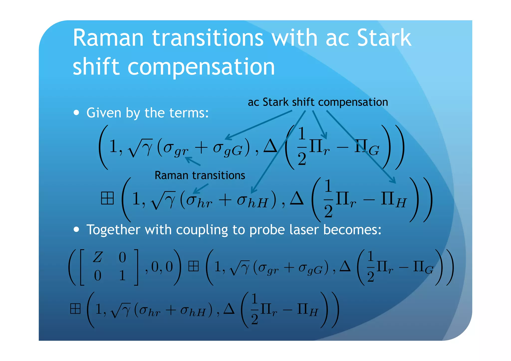
The actual scheme
03.67.Pp,02.30.Yy,42.50.-p,03.65.Yz
quantum error correction
!"
and measurement of syn-
ntral to the modern field of
e. Although substantial work
nsions and refinements of ab-
orts [2, 3, 4] have begun to fo- !#
task of developing implemen- ! "
!!!" $#
ly the fundamental principles
ally accommodate the struc-
!""
models. Such new approaches
$%
quantum memories that make
physical resources and intro-
ted abstractions for quantum !""
plement those we have inher-
r science. !%
recently proposed [5] a cavity
cavity QED) implementation
ty measurement required for
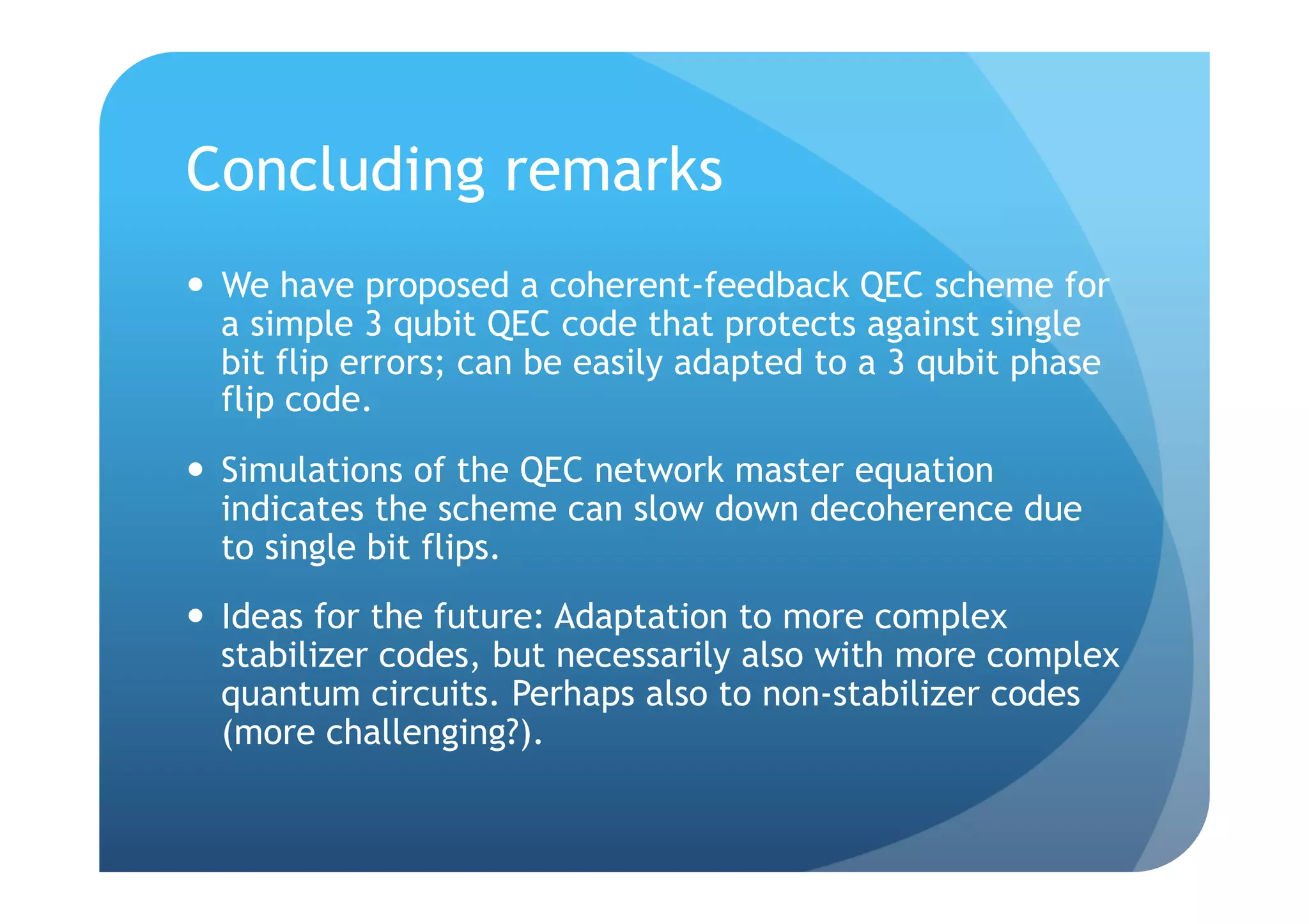
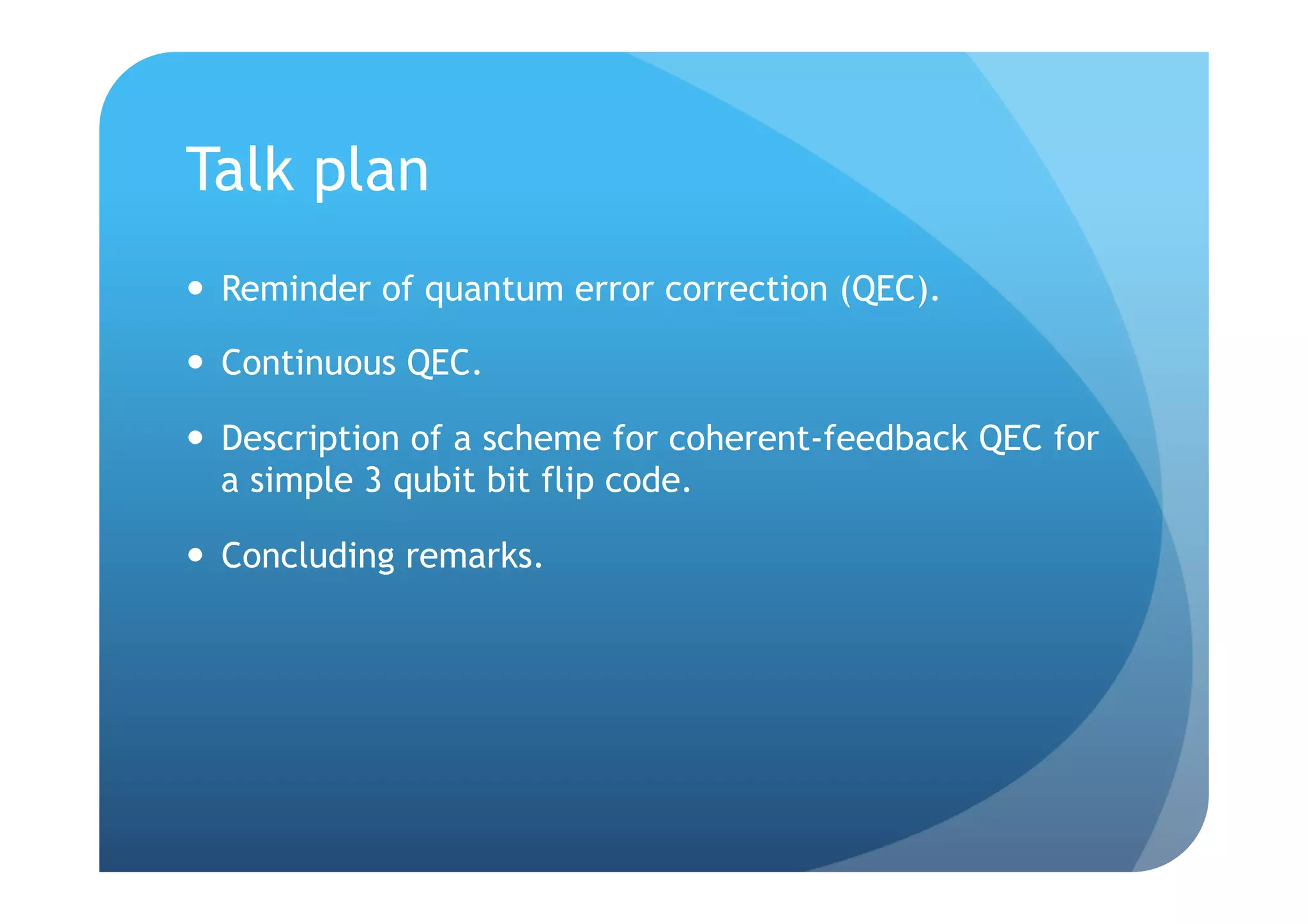
FIG. 1: Schematic diagram of a coherent-feedback quantum
9, 10, 11, 12] versionQuantummemory showing qubits-in-cavities (Q1,facilitate switching
 of the switches R1, R2 inserted to Q2 and Q3), circula- to higher
or phase-flip codes, which be-
amplitude bit flip correcting Raman lasers. (R1 and R2).
tors, beam-splitters, steering mirrors and relays
el in a strong coupling limit. The calculation we present is based on a modified arrange-
further step of describing co- ment that leads to the same closed-loop master equation but
hat realize quantum memories factorizes into four simple sub-networks.
e encoded qubit is suppressed

14. Qubit atomic level scheme
! !"" !!" !
!#"
!
!$"
!&" !%"

15. Raman transitions with ac Stark
shift compensation
ac Stark shift compensation
 Given by the terms:
√ 1
1, γ (σgr + σgG ) , ∆ Πr − ΠG
2
Raman transitions
√ 1
1, γ (σhr + σhH ) , ∆ Πr − ΠH
2
 Together with coupling to probe laser becomes:
Z 0 √ 1
, 0, 0 1, γ (σgr + σgG ) , ∆ Πr − ΠG
0 1 2
√ 1
1, γ (σhr + σhH ) , ∆ Πr − ΠH
2

16. QSDE model for switch/relay
(+* (,* $%#!&'
!"# ()*
!!"
-%$%#!&' !"#
-%$%#!&' !""
- -
$%#!&'
$%# &' !"#
34516
012
.!/%- .!/%-
&' &' !"# !$" !#"
• Simple QSDE model:
Πg −Πh βΠg Πh −σhg
, ,0 , 0, 0
−Πh Πg −βΠh −σgh Πg
Detailed physical model: H. Mabuchi, arXiv:0907.2720

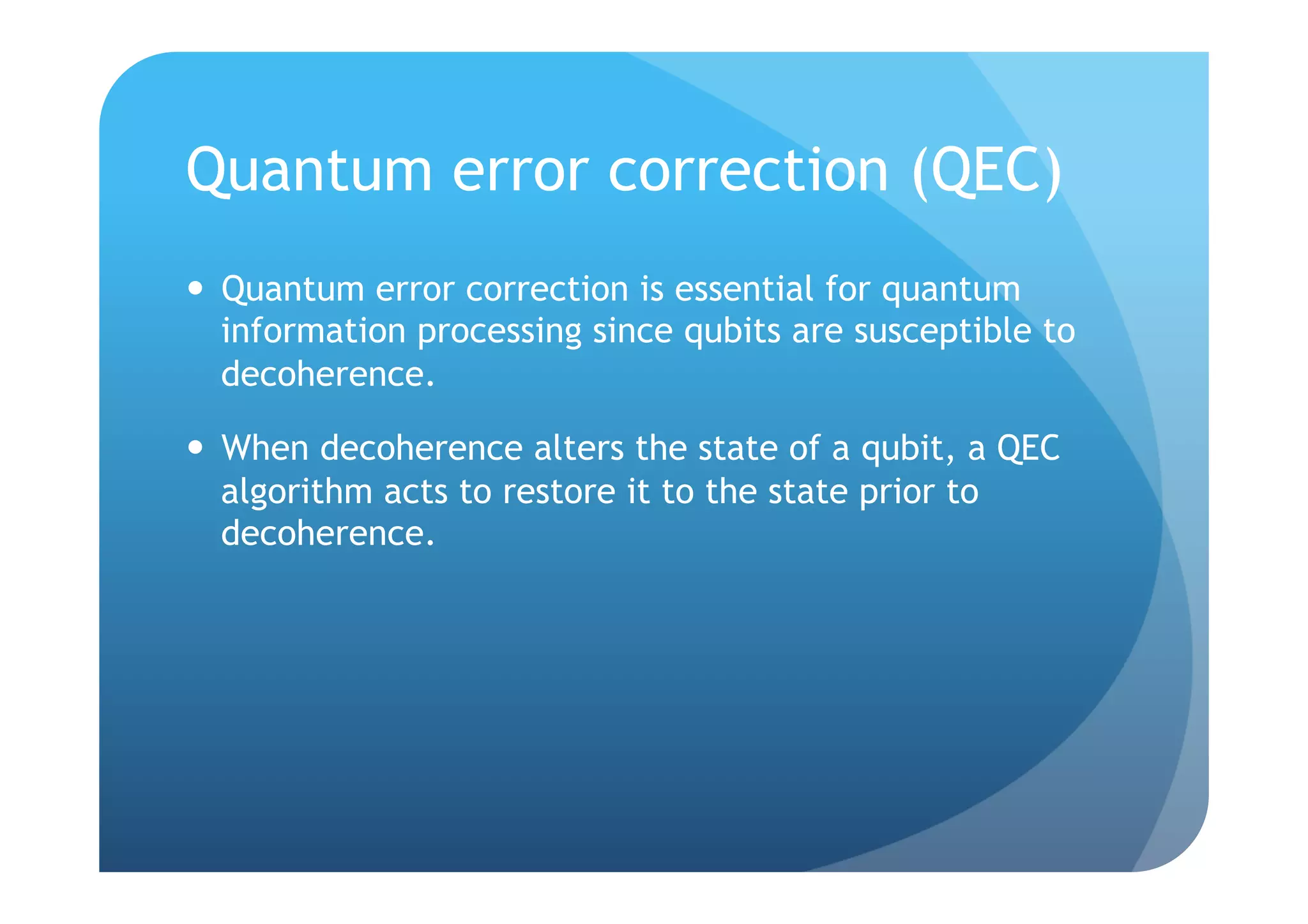
17. QEC network description
!"
 (Modified) half network diagram 3
(+* (,* $%#!&'
!"# ()*
!!" ;88
!# -88 9:
! "
!!!" $#
-%$%#!&' !"#
-%$%#!&' !""
- -
$%#!&'
$%# &' 9< -87 ;8<
!"#
34516
!""
012
$%
.!/%- .!/%-
&' &' !"# !$" !#"
;77
!""
( * ( * ( * ;78
&' !!! "
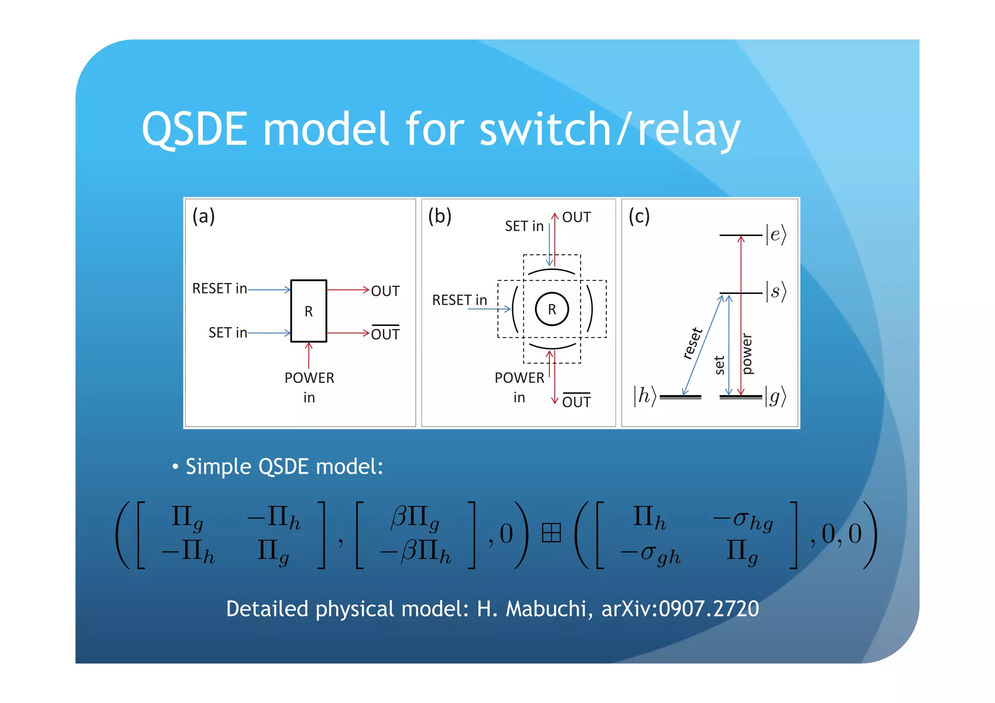
FIG. 3: Details of the ‘set-reset flip-flop cross-over relay’ com- 98
!%
ponent model [22]: (a) input and output ports, (b) coupling
of input/output fields to resonant modes of two cavities, and
!"#7 ;<7
&
(c) relay internal level diagram.
Half it would be possible to f (p=probe path, f=feedback path):
but in a practical implementation network Gp G FIG. 4: Signal-flow diagram of the half-network Gp Gf .
utilize double-pole double-throw relays that switch not
Gp = R12 B3 ((Q we Q21 ) (1, 0, 0)) B1 ,
only the Raman beam itself but also an auxiliary beam 13 proceed to assemble the full network√model N =
Gp Gf G Gf G . Here GΓ = ( ΓX , 0, 0)
Gf = (Q11 chosen soQ22√ΓX (B0) p 2√ΓX0,0,Γ0) describes bit-flip 1decoher-
whose frequency, polarization and amplitude is Q
32 (
) , 0, 5 ( (1, , 0))
that it provides equivalent compensation. 2 3
Some details of our relay model are displayed in (1, 0, 0))
(R11 Fig. 3 ence of the register qubits, and the component connec-
[22]. In electrical engineering parlance, the devices we tions for Gp Gf are shown in Fig. 4 (note that as the
utilize correspond to open quantum systems versions of a signal routing shown in Fig. 1 yields rather unwieldy
cross-over relay driven by a set-reset flip-flop. Each relay network calculations, we are here adopting a modified

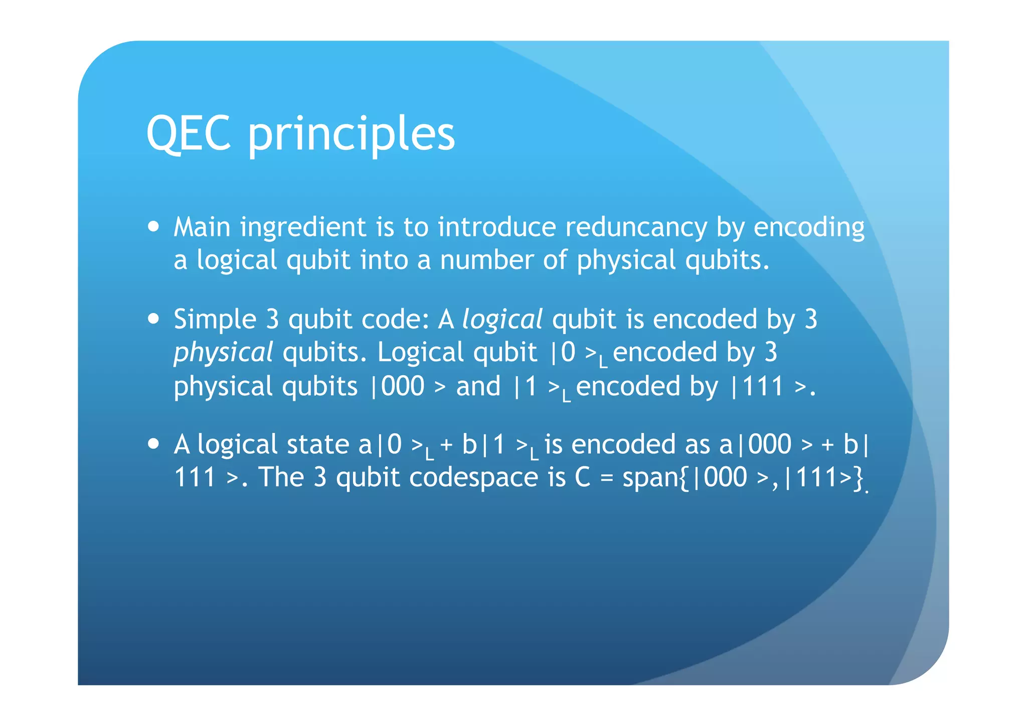
18. QEC network master equation
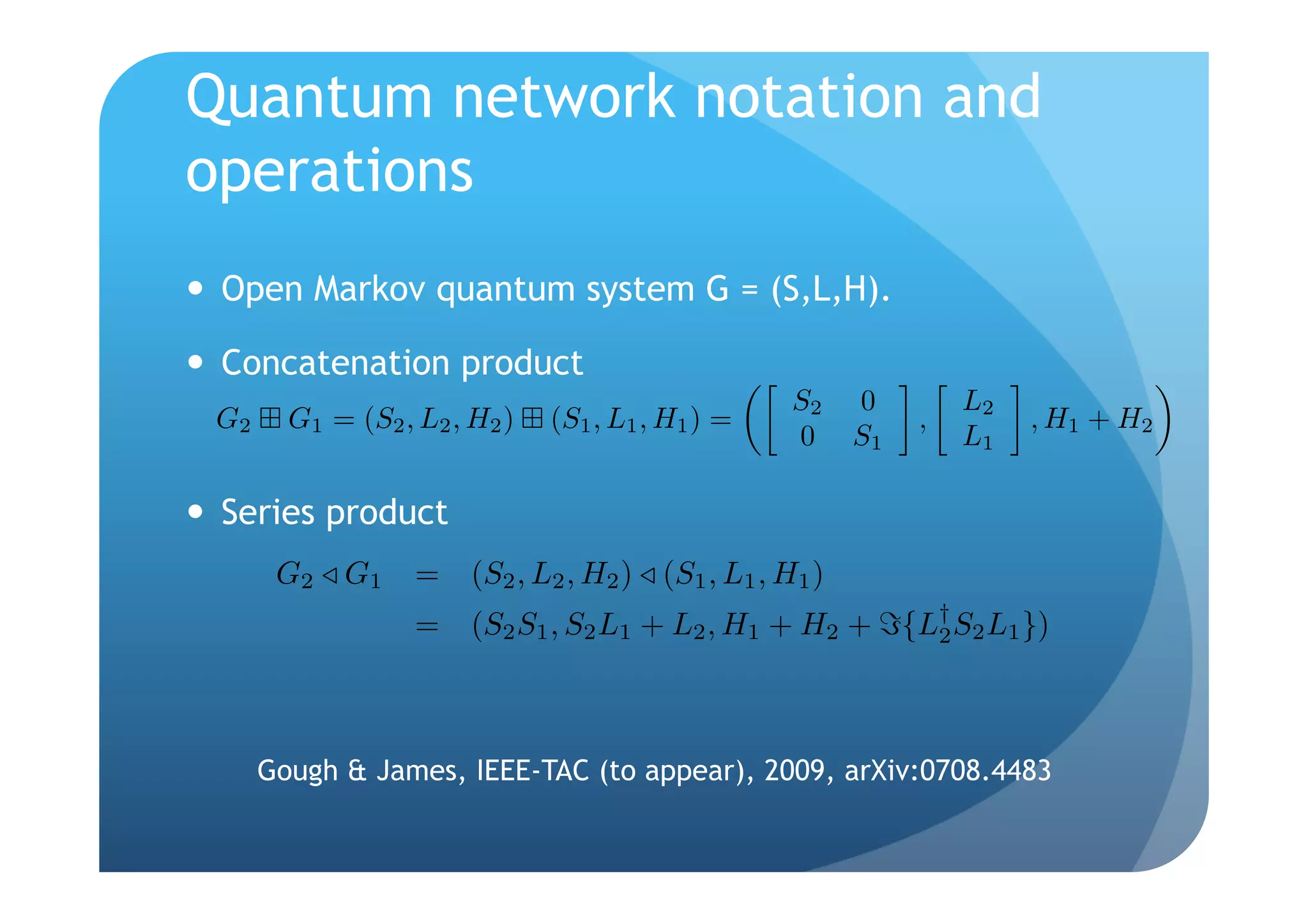
 The QEC network master equation in the limit that Δ, β  ∞
with β2/ Δ constant is:
7
1
ρt = −i[H, ρt ] +
˙ Li ρt L∗ − {L∗ Li , ρt } ,
i=1
i
2 i
where (Ω ≡ β 2 /γ∆),
√ (R2 )
√ (R1 )
H = 2ΩΠ(R1 ) Πh
g X1 + 2ΩΠh Π(R2 ) X3
g
−ΩΠ(R1 ) Π(R2 ) X2 ,
g g
α
L1 = √ σhg 1 ) (1 + Z1 Z2 ) + Π(R1 ) (1 − Z1 Z2 )
(R
h ,
2
α
L2 = √ σgh 1 ) (1 − Z1 Z2 ) + Π(R1 ) (1 + Z1 Z2 )
(R
g ,
2
α
L3 = √ σhg 2 ) (1 + Z3 Z2 ) + Π(R2 ) (1 − Z3 Z2 )
(R
h ,
2
α
L4 = √ σgh 2 ) (1 − Z3 Z2 ) + Π(R2 ) (1 + Z3 Z2 )
(R
g ,
2
√ √ √
L5 = ΓX1 , L6 = ΓX2 , L7 = ΓX3 .

19. Ideal QEC network performance
1
0.995
0.99
Fidelity
0.985
0.98
"=0
"=10
"=30
0.975
"=60
"=90
0.97
0 0.002 0.004 0.006 0.008 0.01
!t
Fidelity = < ψ0 |ρ(t) |ψ0 >; Simulation parameters: Γ = 0.01, α = 10, |ψ0 >
= (| ggg > - |hhh >)/√2; ρ(0) = |ψ0 > < ψ0 |.

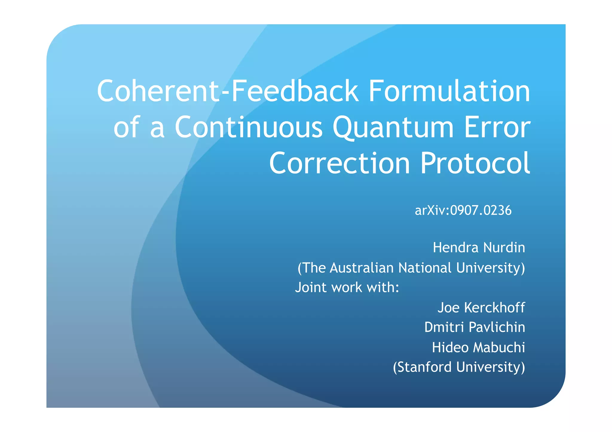
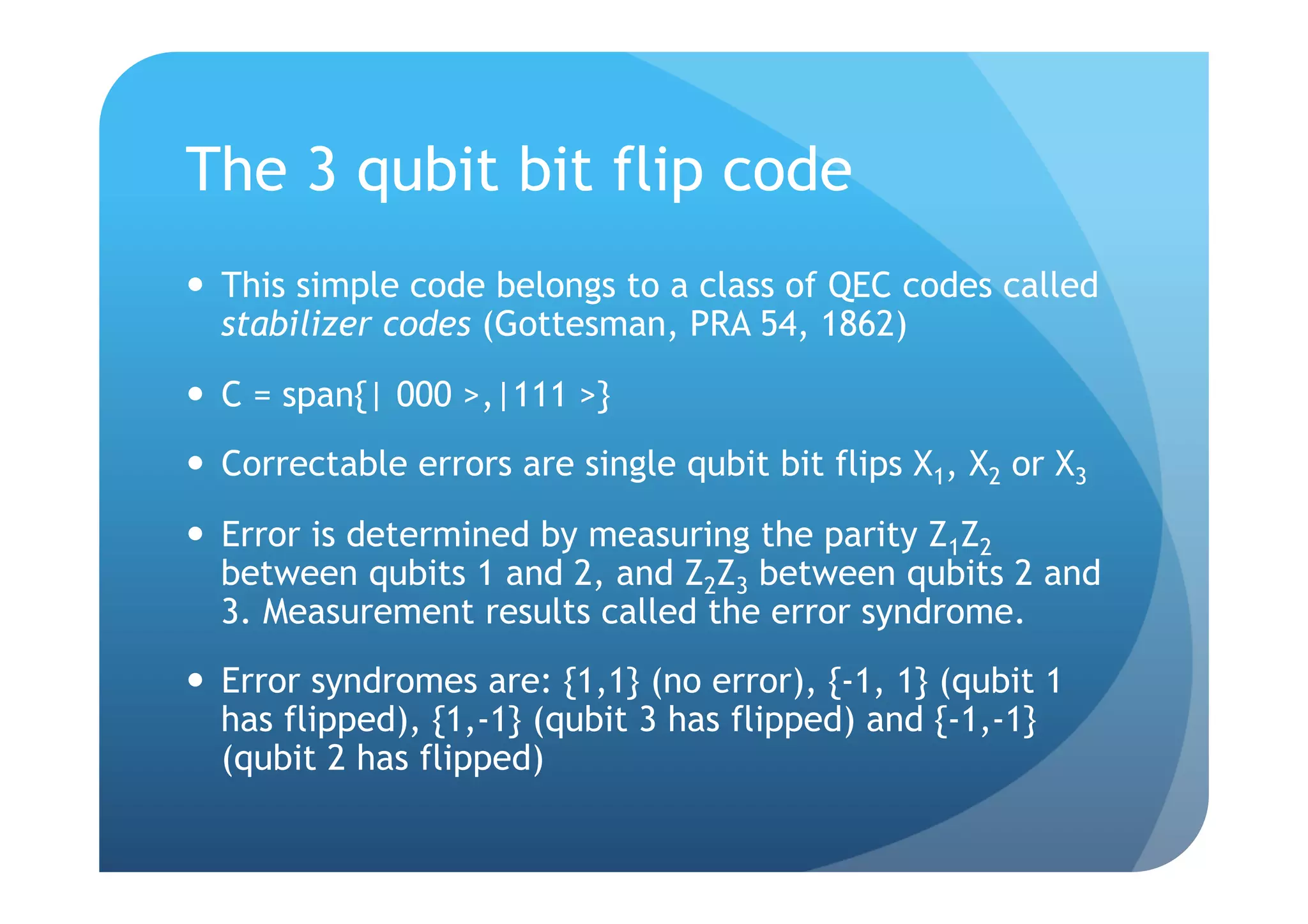
20. Ideal QEC network performance
-./01234,2540167819:4/28;<4!=>! *+,-./0-1213,.41156)/78.!9:!
"#&' "#'$!$
"#&+
"#'$!%
"#&*
"#&$
"#'$!%
"#&%
"#&) "#'$!(
;
?
"#&&
"#'$!(
"#&!
"#&
"#'$!&
"#!(
"#!' "#'$!&
% %
& ! & !
"#$ "#$
" "
" "
!& !&
!"#$ !"#$
"
!% !! !% !!
, " )
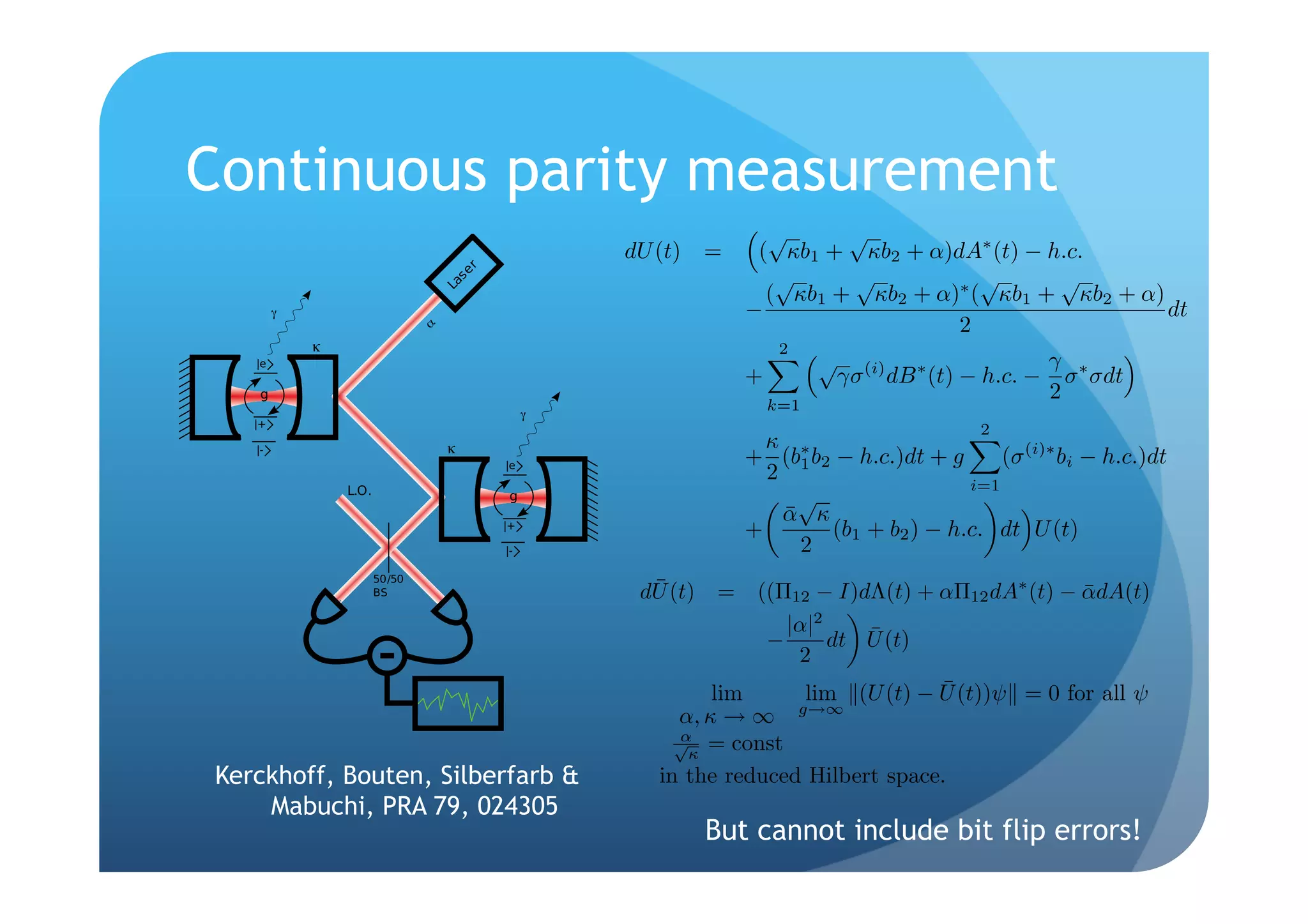
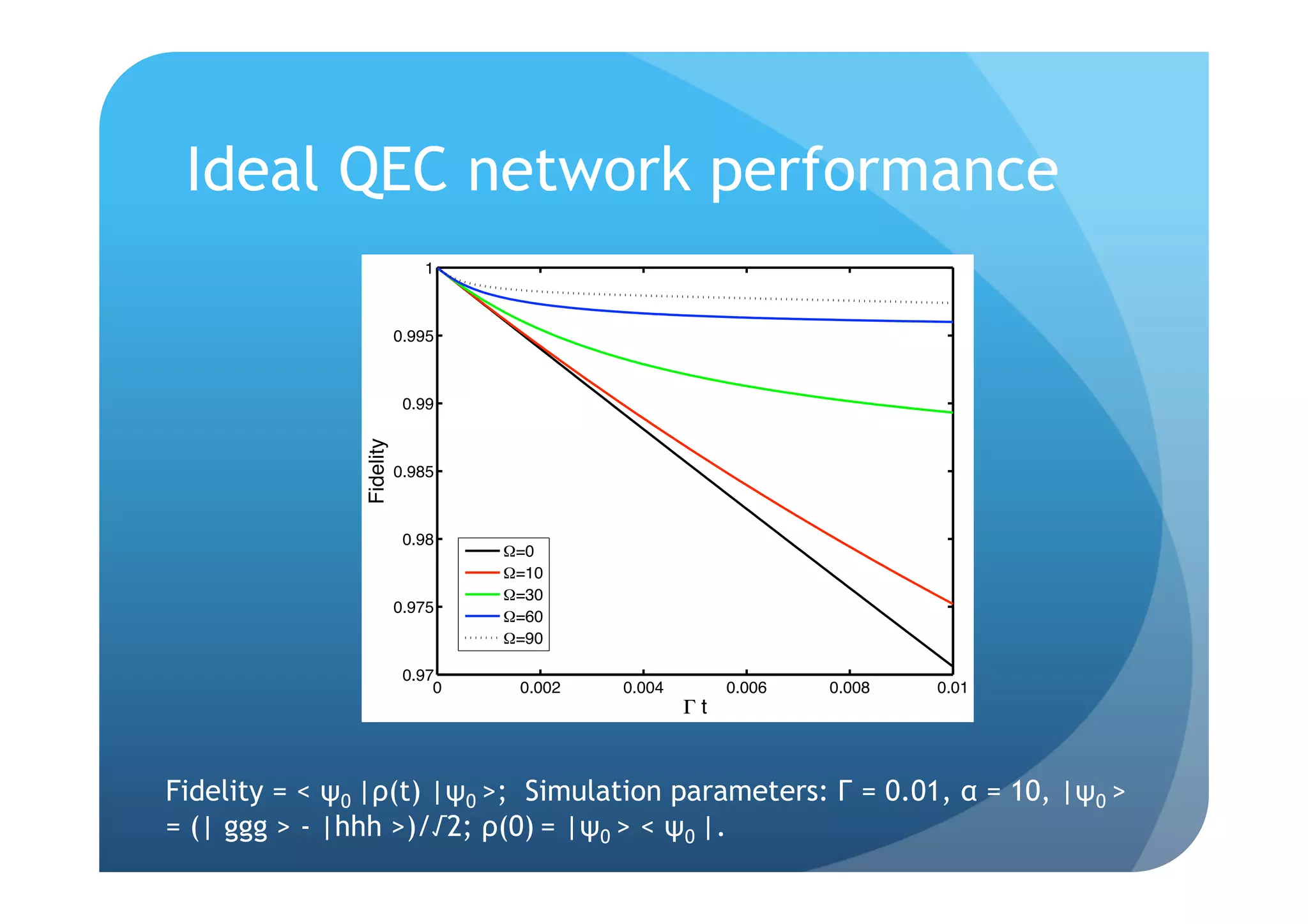
Fidelity = < ψ0 |ρ(T) |ψ0 >; Simulation parameters: Γ = 0.01, α = 10,β = 30,
|ψ0 > = a |ggg > + √(1-a2)eiθ|hhh >, a in [-1,1], θ in [-π,π]; ρ(0) = |ψ0 > < ψ0 |.

21. Concluding remarks
 We have proposed a coherent-feedback QEC scheme for
a simple 3 qubit QEC code that protects against single
bit flip errors; can be easily adapted to a 3 qubit phase
flip code.
 Simulations of the QEC network master equation
indicates the scheme can slow down decoherence due
to single bit flips.
 Ideas for the future: Adaptation to more complex
stabilizer codes, but necessarily also with more complex
quantum circuits. Perhaps also to non-stabilizer codes
(more challenging?).