The document discusses how to use Excel as a database by structuring data in a list format. Key points include: - Excel lists consist of columns and rows of data with each column containing the same type of data and each row containing a full set of data. - Excel lists allow you to sort, filter, and analyze data similarly to a database through features like sorting, filtering, and advanced filtering. - Additional techniques like custom sorting, forms, and numbering rows enable more advanced database-like functions in Excel.

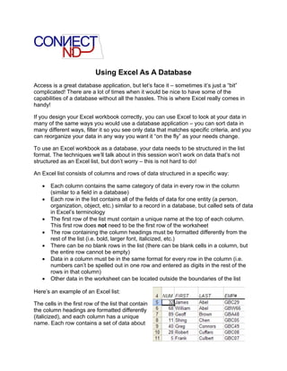
1. Using Excel As A Database
Access is a great database application, but let’s face it – sometimes it’s just a “bit”
complicated! There are a lot of times when it would be nice to have some of the
capabilities of a database without all the hassles. This is where Excel really comes in
handy!
If you design your Excel workbook correctly, you can use Excel to look at your data in
many of the same ways you would use a database application – you can sort data in
many different ways, filter it so you see only data that matches specific criteria, and you
can reorganize your data in any way you want it “on the fly” as your needs change.
To use an Excel workbook as a database, your data needs to be structured in the list
format. The techniques we’ll talk about in this session won’t work on data that’s not
structured as an Excel list, but don’t worry – this is not hard to do!
An Excel list consists of columns and rows of data structured in a specific way:
• Each column contains the same category of data in every row in the column
(similar to a field in a database)
• Each row in the list contains all of the fields of data for one entity (a person,
organization, object, etc.) similar to a record in a database, but called sets of data
in Excel’s terminology
• The first row of the list must contain a unique name at the top of each column.
This first row does not need to be the first row of the worksheet
• The row containing the column headings must be formatted differently from the
rest of the list (i.e. bold, larger font, italicized, etc.)
• There can be no blank rows in the list (there can be blank cells in a column, but
the entire row cannot be empty)
• Data in a column must be in the same format for every row in the column (i.e.
numbers can’t be spelled out in one row and entered as digits in the rest of the
rows in that column)
• Other data in the worksheet can be located outside the boundaries of the list
Here’s an example of an Excel list:
The cells in the first row of the list that contain
the column headings are formatted differently
(italicized), and each column has a unique
name. Each row contains a set of data about

2. one person, and there are no blank rows in the list.
Data can be sorted alphabetically or numerically in Excel using the Quick
Sort buttons on the Standard Toolbar. Sorts can be in Ascending (A-Z) or
Descending (Z-A) order.
Many people get frustrated with sorting in Excel
because of the way they perform the sort – first they
select an entire column by clicking on the column letter,
then they click the Quick Sort buttons on the Toolbar.
The only trouble with this method is that only the
selected data gets sorted – the rest of the data in each
row stays right where it started!
To sort the right way in Excel, all you need to do is put
the cell pointer in any cell in the column you wish to
sort, then click one of the Sort buttons.
If your data wasn’t originally sorted alphabetically or numerically, once you’ve performed
a sort on the data you won’t be able to return the list to its original order; however, you
CAN add an additional column to your list, and number each row sequentially so that
you can resort that column numerically.
You can use Excel’s Fill Series feature to quickly number the new column sequentially:
1. In the first cell to be numbered, type the number 1
2. In the next cell down, type the number 2
3. Select those two cells
4. Position the mouse pointer over the Fill Handle in the lower
right corner of the selected cells
5. Click and drag the black, thin cross mouse pointer down to the
end of the column
6. To return the list to its original sort order, select any cell in the
numbered column and click the Sort Ascending button
The Quick Sort buttons only allow you to perform sorts on one column at a time, but
sometimes you need to perform more complex sorts. For example, if you have a list of
names you may want to sort first by Last Name, then additionally by First Name in case
there are duplicate last names.
Use the Data, Sort command to perform this type of sort and others. Place the cell
pointer in any cell in the list, choose Data from the Menu Bar, then click Sort…

3. In the Sort dialog box, select the column you
wish to use as the primary sort criteria from the
Sort By drop-down list. Additionally, you can
select a secondary sort criteria from the first
Then by drop-down list and a third criteria from
the second Then by drop-down list. This sorting
method should make your sorting tasks much
easier!
There are times when the default Sort options just don’t fit – for example, what
if you need to sort sets of data in chronological order by Month? Excel’s default
sort methods sort either alphabetically or numerically, not chronologically.
You can force Excel to sort a list in other ways by using Excel’s Custom Lists
feature. Excel already has a few built-in Custom Lists you can use, but you can
also build your own Custom Lists to suit your needs.
To sort an Excel list chronologically
by month, place the cell pointer in any cell in
the column you want to sort, then select
Data, Sort as you normally would and select
your Sort criteria. Before you click OK, click
the Options button.
In the Sort Options dialog box,
select the January, February,
March entry from the First key
sort order drop-down list and
click OK. Next, Click OK to
close the Sort dialog box. Your
list should now be sorted in
chronological order!

4. If you don’t see a built-in Custom List that meets your needs you can build your own:
1. On the Menu Bar, select Tools, then
click Options
2. At the top of the Options dialog box,
click the Custom Lists tab to select it
3. In the Options dialog box create a new
list by typing each entry in the List
entries: text box in the order you want
the list to be sorted – placing each entry
on a separate line
4. Click the Add button, then click OK. You
only have to create your Custom List
once
You can use any of the entries in the Custom lists: text box as the First key sort order in
the Sort Options dialog box to perform a custom sort.
When your worksheet is structured as an Excel list, you can use the Data command to
filter items that meet criteria you specify. When you’ve filtered a list, rows of data that
don’t match your criteria are temporarily hidden from view, but not deleted, making it
easier to find exactly what you’re looking for and do different kinds of data analysis.
There are two methods of filtering an Excel list – AutoFilter and Advanced Filter.
AutoFilter is easier to use than the Advanced Filter method, but the AutoFilter method
doesn’t always have the power you need. Try AutoFiltering first – if that doesn’t meet
your filter needs, you can always remove the AutoFilter, and try building an Advanced
filter.
To turn on AutoFilter, place the cell pointer in any
cell within your list, click Data, highlight Filter, then
click AutoFilter. Your list now displays small black
triangles next to each column heading.
When you click a triangle in one column, a list
of all of the different values in that column
drops down. Click the desired value to filter
the list to display only those values.

5. When a filter is applied, the column
that is filtered shows a blue triangle
rather than a black triangle and the
row numbers at the left side of the
worksheet don’t display rows that
have been filtered out.
If you’ve already applied one filter, you can further refine your filter by setting up a
logical condition known as an AND condition. An AND condition means that in order to
be selected in the filter, a set of data has to meet BOTH conditions specified. For
example, if you wanted to see all of the employees working in the Maine Division who
work 40 hours per week, you could select Maine as the first condition in the DIVISION
column and 40 as the second condition in the HRS column (Maine AND 40):
You can also filter lists for ranges of values using Custom filters and wildcard characters
in the AutoFilter. To use a Custom filter, click the triangle for the column you wish to
filter and choose (Custom…) from the drop-down list.
In the Custom AutoFilter dialog box
you can specify a range of values by
choosing a different operator than
“equals” from the Show rows where …
drop-down list:
In this example, only those employees
who worked less than 40 hours per
week would be selected in the filter.
Wildcard characters are special characters
used to match all records that meet the
specified pattern of characters. For example,
to find all employees whose last names begin
with the letter S use the asterisk * wildcard
character after the letter S in the Custom
AutoFilter dialog box:

6. When the AutoFilter feature just doesn’t meet your needs, turn off AutoFiltering and use
the Advanced Filter method to specify more complex criteria. To remove the filter so all
of the data is displayed, place the cell pointer in any cell in the list, click Data, highlight
Filter, then click AutoFilter. All of the triangles will disappear and any filtered data will
reappear.
For example, suppose you’d like to display the records for any employees who work in
the Sales Dept in the Maine Division and any employees who work in the Research
Dept in the Vermont Division. No matter what you do, you can’t make this more complex
filter work using AutoFilter. This criteria uses two AND conditions and an OR condition:
(Sales Dept AND Maine Division OR Research Dept AND Vermont Division). An OR
condition specifies that a set of data needs to meet only one of the conditions in order to
be included in the results.
To use an Advanced Filter, first you’ll need to define a
criteria range in another area of your worksheet outside the
boundaries of your list. A criteria range specifies the criteria
and conditions like this: criteria placed horizontally in the
range produce an AND condition, criteria placed vertically in
the range produce an OR condition. Here’s the criteria range
to use for the example above:
The first row of the criteria range must contain the names of the columns you want to
filter on. This example’s criteria range is located outside of the list in the range M1:N3
and reads “Research AND Vermont OR Sales AND Maine (Excel is not case-sensitive).
Next, place the cell pointer in any cell within the list, click Data, highlight Filter, then click
Advanced Filter. In the Advanced Filter dialog box type the range where you placed
your criteria in the Criteria range: text box (i.e. M1:N3). Check the cell references
specified in the List range: text box to make sure the correct list area is selected, then
click OK – and Voila! -- only sets of data that meet your criteria should be displayed.
There’s one more little-known feature in
Excel that can make your work a LOT easier.
You can speed up data entry into an Excel
list by using the Form feature.
Place the cell pointer in any cell within the
list, select Data, then click Form…
You’ll see a dialog box on screen that
contains a text box for every column in your
list.
To create a new set of data, click the New
button then type data into a field and press
the Tab key to move to the next field. When
you reach the bottom of the form and press
AND
O
R

7. the Tab or Enter key, you move to the next set of data to enter more data.
You can also use the Form feature to quickly locate a specific set of data by clicking the
Criteria button, then specifying the criteria to search for in the appropriate field. When a
set of data matches your criteria, that data is displayed in the form window.
Now that you’ve seen how useful and powerful an Excel list can be, you may want to
structure all of your Excel worksheets as lists – it can be quite a time-saver when you
need it!