SlideShare a Scribd company logo
1 of 103
Download to read offline
Mr. T.SOMASUNDARAM
DEPT OF MANAGEMENT
KRISTU JAYANTI COLLEGE
BENGALURU
UNIT – 4
IN BUSINESS
UNIT – 4
SPREADSHEET IN BUSINESS
Introduction to Spreadsheet, Features of Spreadsheet,
Cell reference, Format cells, Data Validation,
Protecting Sheets, Data Analysis in Excel: Sort, Filter,
Conditional Formatting, Preparing Charts, Pivot
Table, What if Analysis (Goal seek, Scenario manager),
Financial Functions: NPV, PMT, PV, FV, Rate, IRR,
DB, SLN, SYD. Logical Functions: IF, AND, OR,
Lookup Functions: V Lookup, H Lookup,
Mathematical functions and text functions
Introduction to Spreadsheet
Microsoft Excel is spreadsheet software in the Microsoft Office
Suite widely used to perform mathematical calculations.
The data is spread in a tabular form consisting of rows and
columns.
It provides built-in features and tools such as formulas, functions
and data analysis tools that make it easier to work with large
amount of data.
It allows to store, organize and analyse numerical and text data.
A file of MS-Excel is called a Workbook and it contains multiple
worksheets or spreadsheets primarily used to work with numbers
and text.
A worksheet is the grid of cells where you can type the data.
Definition:
“A Spreadsheet is a file that exists of cells in rows and
columns and can help to arrange, calculate and sort data”.
MS-Excel helps us to –
Arrange data in an organized way.
Perform calculations.
Compare data through charts.
Sort data for better analysis.
Compare two workbooks side by side.
Features of MS-Excel:
Some of the main features of MS-Excel are –
Excel provides support for multiple sheets within a workbook.
It provides a standard grid, which may be scrolled and
zoomed.
Text, numeric or date values or formulas may be entered into
selected cell through formula bar at the top of screen.
A worksheet may be selected simply by tapping on it & can
create or delete or rename existing worksheets.
Cells may be formatted using format pages, specify font style,
borders, text and background colours, size of cells and text
alignment.
Features of MS-Excel:
Excel provides the ability to search worksheet for any phrase,
number or other text, letting you easily scroll between search
results.
Excel supports a variety of functions used to perform basic
calculations based on parameters set by user.
Spreadsheets can be integrated for use with other software
programs. (E.g.) Mail merge
Professional looking graphs and charts can be created very
quickly from a range of data which allows you to view the data
pictorially.
Easy to make changes and corrections to data on the worksheet.
Spreadsheet (Excel) Elements or Terms
1. File Tab – it helps you to manage the Microsoft application and provide
access to its options such as Open, New Save, As Print, etc.
2. Quick Access Toolbar – displays quick access to commonly used
commands.
3. Ribbon – displays groups of related commands within tabs. Each tabs
provides buttons for commands.
4. Tabs – it appears across the top of the Ribbon and contain groups of
related commands. (E.g.) Home, Insert and Page Layout.
5. Title Bar – displays the name of the application file or document title.
6. Search Bar – advance search will help you find and perform tasks.
7. Name box – displays the active cell location.
8. Cell – intersection of a row and column, cells are always named with
Spreadsheet (Excel) Elements or Terms
9. Formula Bar – displays the address of the active cell on the left edge
and it also shows the current cell’s contents.
10. Status Bar – displays information about the current worksheet.
11. Zoom control – use to zoom the excel screen in or out by dragging
the slider.
12. View Button or Option – displays worksheet view mode like normal
layout view or page layout view or page break view.
13. Sheet Area – the area where you enter the data.
14. Row Bar – rows are numbered from 1 onwards and keeps on
increasing as you keep entering data.
15. Column Bar – columns are numbered from A onwards and keeps on
increasing as you keep entering data.
Spreadsheet (Excel) Screen
Spreadsheet (Excel) Shortcuts
Cell Reference
Cell Referencing:
The cell address in a formula is known as the cell reference.
With the help of cell references, you can use the data in different
parts of a worksheet.
Types of cell referencing:
1. Relative Reference:
When you create a formula, references to cell(s) are usually
based on the position relative to the cell. When you copy or
move a formula to other cells, the reference cell automatically
changes.
(E.g.) In the below figure, the formula in A3 cell is = A1 + A2.
When you copy the formula from A3 cell to B3 cell, excel
automatically changes the reference cell to match the location of
cells. (i.e.) B3 cell is = B1 + B2.
Cell Reference
2. Absolute Reference:
Absolute reference is used when you do not want to change
the address of the cell on copying the formula to another cell.
For this purpose, you have to add the dollar symbol ($) before
the column and the row number.
(E.g.) In the below figure, enter the numbers you want to
calculate in B2 cell and B3 cell. Create a simple formula =
B2+B3 in B5 cell.
To create an absolute reference in the formula, insert a $ symbol
before the B (column reference) and 2 (row reference) in
reference to B2, so new formula is =$B$2+B3.
Copy and Paste the formula to another adjacent cell D5. The
formula now includes absolute reference to B2, (=$B$2+D3)
Cell Reference
3. Mixed Reference:
It is a combination of Relative and Absolute reference. In this
type of reference, either row or column has to remain fixed.
(E.g.) In the below figure, enter the numbers you want to
calculate in A1 cell and A2 cell. Create a simple formula =
A1+A2 in A3 cell.
To create a mixed reference in the formula, insert a $ symbol
before the A (column reference) for A1 cell and 2 (row
reference) in reference to A2 cell, so new formula is =$A1+A$2.
Copy and Paste the formula to another adjacent cell B3. The
formula now includes absolute reference to B3, (=$A1+B$2)
Format Cells
Once the data have entered into a worksheet, we need to
format it in different ways like -
Format Text in Bold or Italics
Format Text as underlined
Change the Font Style
Change the Font Size
Change the Text Colour
Add a Border
Add a fill colour
Column Width
Row height
Insert / Delete Rows
Insert / Delete Columns
Wrap Text
Merge Cells
Data Validation
Data Validation is an important task and to restrict data entry to certain
range of dates, limit choices by using a list, entering only whole
numbers, etc.
It provides instructions to users and clear messages when invalid data is
entered is also essential to make the data entry experience go smoothly.
Protecting Sheets
To prevent others users from accidentally or deliberately changing,
moving or deleting data in a worksheet, we can lock the excel
worksheet and then protect the sheet with a password.
The two step process are –
Step 1: Unlock any cells that
needs to be editable.
Step 2: Protect the worksheet
& allow the users of this
Worksheet to list, select the
Elements what you want people
to be able to change.
Data Analysis in Excel
Sorting or Data Sorting:
Sorting or Data Sorting is a common spreadsheet task that
allows you to easily reorder your data. The most common type
of sorting is alphabetical ordering, which you can do in
ascending or descending order.
To Sort in Alphabetical Order:
Select a cell in the column you want to sort.
Click the Sort & Filter command in the Editing group on the
Home tab. Select Sort A to Z.
Now, the data in the spreadsheet will be organized
alphabetically.
Sort in Alphabetical Order
Data Analysis in Excel
To Sort in Numerical Order:
Select a cell in the column you want to sort.
Click the Sort & Filter command in the Editing group
on the Home tab. Select Smallest to Largest.
Now, the data in the spreadsheet will be organized
numerically from the smallest to largest value.
Sort in Numerical Order
Data Analysis in Excel
To Sort by Date or Time:
Select a cell in the column you want to sort.
Click the Sort & Filter command in the Editing group
on the Home tab. Select Sort Oldest to Newest.
Now, the data in the spreadsheet will be organized by
date or time.
Sort by date or time
Data Analysis in Excel
Filtering:
Filtering is a convenient and reliable way to locate and
manage spreadsheet data. This allows you to focus on specific
spreadsheet entries. Filtered data can be copied, manipulated and
printed without having to move it to a new spreadsheet.
Data Filtering in Excel enables the user to work with a subset
of data within the data list. When filter is created, only the
records that contain the values specified are displayed. Other
records in the data list are hidden temporarily.
To Filter Data:
Open the spreadsheet in which you want to filter data.
Prepare your data for an Excel Auto filter.
Select any cell within the range that you would like to filter.
Select Filter Command in Sort & Filter group under Data tab.
Drop down arrows will appear at the top of each column range.
Click the drop-down arrow of the column containing the desired
criteria to be filtered.
To filter the data by criteria, click to clear the Select All check box and
all other boxes will be cleared.
Click to Select the check boxes of criteria that you want to appear in the
filtered list.
Click OK to filter the range by selected criteria.
Data Analysis in Excel
Conditional Formatting:
A format, such as cell shading or font colour, that Excel
automatically applies to cells if a specified condition is true.
Conditional Formatting is a special formatting feature of excel
that sets a cell’s format according to condition that you
specify.
Conditional Formatting allows you to present numeric data in
different colours. (E.g.) you can shade data depending on
whether the value is greater, equal to, or less than zero.
Conditional Formatting:
Open the spreadsheet and type the data in cells.
Select the range of particular data.
In Home Tab, under Styles group, Click Conditional
Formatting command. A drop down list will be displayed.
Click Highlight Cells Rules – Greater Than.
Greater than dialog box will be appeared.
Enter the value in any field (Greater or Less than or Equal to)
and select colour fill field option from “with: drop down list”.
Click OK.
The final result of conditional formatting will appear.
Data Analysis in Excel
Preparing Charts:
Charts (also known as graphs) are a visual representation of
data in a worksheet.
Charts allow you to present data entered into the worksheet in
a visual format using a variety of graph types.
Charts make it easy to see comparisons, patterns and trends in
data.
Components of a Chart:
1. Source Data - this is range of cells that make up a chart.
2. Title – this is the title of the chart.
3. Legend - this is the chart key, which describes what each
colour on the chart represents.
4. Axis – this is vertical and horizontal parts of a chart. The
vertical axis is often referred to as the Y axis, while the
horizontal axis is referred to as the X axis.
5. Data Series – this is the actual charted values, which usually
are rows or columns of the source data.
6. Value Axis – this is the axis that represents the values or units
of the source data.
7. Category Axis – this is the axis identifying each data series.
Types of Charts:
1. Area Chart:
Area chart emphasizes the trend
of each value over time. An
area chart also shows the
relationship of parts to a whole.
2. Column Chart:
Column chart uses vertical bars
or columns to represent data. They
can work with many different
types of data.
3. Bar Chart:
Bar chart is similar to a column chart
except these use horizontal instead of
vertical bars. The bar chart shows
variations in value over time.
4. Line Chart:
Line chart shows trends and
variations in data over time. Line chart
displays a series of points, called data
points, that are connected with lines
and see whether values are increasing
or decreasing over time.
5. Pie Chart:
Pie Chart displays the contribution of each value to the total. Pie chart
are very effective way to display information when you want to
represent different parts of the whole or percentages of a total.
In Pie Chart, each value is shown as a slice of the pie, so it is easy to
see which values make up the percentage of a whole.
To create Chart:
First of all, enter the data into the worksheet and highlight all cell that
will included in chart including column titles and row labels.
Select the source data for the chart.
Click the Insert tab. Select desired chart category.
The chart will appear in the worksheet.
To change chart types, Select the chart and Click the Design Tab. In
Type group, click the Change Chart Type command.
Change Chart type dialog box appears.
Select the desired chart type, and then Click OK.
Data Analysis in Excel
Pivot Table:
Pivot tables are interactive tables that allow the user to group
and summarize large amounts of data in a concise, tabular
format for easier reporting and analysis.
They can sort, count and total the data, and are available in a
variety of spreadsheet programs.
Pivot table allows you to summarize your data more quickly
and with more flexibility.
Pivot tables are great way to summarize, analyze, explore and
present your data and you can create them with just a few
clicks.
To create a Pivot Table:
Select the Table or Cells, including column headers containing data you
want to use.
Click Insert Tab --- Tables group --- Pivot Table command.
Select Pivot Table option from drop down list.
Create Pivot table dialog box will appear. Make sure settings are
correct, then Click OK.
A blank Pivot Table will appear on left, Field list will appear on right
side of worksheet.
To Add Fields to Pivot Table – according to requirements, we have to
decide which fields to add to Pivot Table. Each field is a column header
from source data.
To Change Row Labels – drag any existing field out of Row labers, and
it will disappear.
Data Analysis in Excel
What if Analysis:
It is a tool that enables you to find the input values needed to
achieve a goal or objective.
Goal Seek Feature:
Goal seek feature allows you to change the data used in a
formula in order to find out what results will be.
To use Goal Seek, select the cell containing formula that will
return the result you are seeking and then indicate the target
value you want the formula to return and location of input
value that Excel can change to reach the target.
To use Goal Seek:
Select the cell containing the formula that will return the result you are
seeking.
On the Data tab, Choose What-if Analysis ----- Goal seek in the Data
Tools group.
Goal Seek Dialog box will open. Cell is active cell when you open this
dialog box, Set cell text box already contains the cell reference (E.g.)
C1.
Select the To Value text box and enter the goal. This is the value you
want the formula in Set Cell box to reach.
Select By changing cell text box and select cell that you want to
change.
Click OK and it displays Goal Seek status dialog box along with the
results.
Scenario Manager:
The use of Scenario Manager in Excel allows you to have a
certain set of inputs and outputs for a “Scenario”, and then lets
you view different scenarios of outputs as the inputs change.
This can help give people information to make decisions on
their business based on different outcomes displayed by
Scenario Manager.
Excel’s Scenario Manager lets you create and save sets of
different input values that produce different calculated results
as named scenarios.
The key to creating various scenarios for table is to identify
various cells in data whose values can vary in each scenario.
To use Scenario Manager:
Open the spreadsheet containing the data for which you want to create
scenario.
On the Data tab of Ribbon, Choose What-If Analysis ----- Scenario
Manager in the Data Tools group.
The Scenario Manager dialog box appears.
To create a Scenario, Click the Add button. Add Scenario dialog box
appears.
Type the name of scenario in Scenario name text box, specify the
Changing Cells, Click OK.
Excel displays the Scenario Values dialog box.
Enter the values for each of changing cells in the text boxes.
Click on Add button. Excel redisplays Add Scenario dialog box.
To use Scenario Manager:
Repeat the steps to enter the other scenarios. When you finish entering
values for the final scenario, click OK instead of Add.
Scenario manager dialog box makes another appearances, this time
displaying the names of all scenarios in its Scenarios list box.
To have Excel plug the changing values from any scenario into the
table, click the scenario name in the Scenarios list box and then Click
Show.
Click the Close button when you are finished with the Scenario
Manager.
Financial Functions
Financial functions calculate financial information, such as net
present value and payments.
(E.g.) Calculate monthly payments required to buy a car at a certain
loan rate using the PMT function.
Some of the commonly used financial functions are –
1. RATE:
The RATE function is used to calculate the interest rate charged on
a loan.
2. NPER:
The NPER function is used to calculate the total number of
periods (months, quarters, years) over which the loan or
investment is to be paid.
3. PMT:
The PMT function calculates the payment for a loan based on
constant payments and a constant interest rate. It includes principal
and interest but no other fees or taxes.
4. PV:
The PV function calculates the present value of a loan or an
investment, based on a constant interest rate.
5. FV:
The FV function calculates the future value of an investment based
on a constant interest rate.
6. NPV:
The NPV function calculates the net present value of an
investment using a discount rate and a series of future cash flows.
7. IRR:
The IRR function returns the internal rate of return for a series of
cash flows that occur at regular intervals.
8. DB:
The DB function returns the depreciation value of an asset during
a mentioned period by using fixed declining balance method.
9. SLN:
The SLN function returns the straight-line depreciation of an asset
for one period.
10. SYD:
The SYD function returns the “sum of years” depreciation for an
asset in a given period.
To Calculate PMT:
PMT Output:
To Calculate PV:
PV Output:
To Calculate NPER:
NPER Output:
To Calculate SLN:
SLN Output:
Logical Functions
Logical functions are used frequently for testing conditions and making
decisions. Some of the commonly used logical functions are –
1. IF:
The IF Function checks whether a condition is met or not. It returns one
value if the condition is TRUE and another value if the condition is
FALSE.
(E.g.) Select Cell C1, enter the function =IF(A1>=33,”PASS”,”FAIL”)
and Press ENTER.
2. AND:
The AND Function returns TRUE if all conditions are true and returns
FALSE if any of the conditions are false.
(E.g.) Select Cell C4, enter the function
=IF(AND(A4>=60,B4<100),”FIRST”,”SECOND”) and Press ENTER.
Here AND function
returns FALSE because
the value in cell A4 is
not greater than or
equal to 60, though the
value in cell B4 is less
than 100. So second
condition is true and
first condition is false.
3. OR:
The OR Function returns TRUE if any of the conditions are TRUE and
returns FALSE if all conditions are false.
(E.g.) Select Cell C8, enter the function
=IF(OR(A8>=60,B8<100),”FIRST”,”SECOND”) and Press ENTER.
Here ORD function
returns TRUE because
the value in cell B4 is
less than 100, though
the value in cell A4 is
not greater than or
equals to 60. So one of
the two condition, one
is true.
Lookup Functions
The lookup and reference functions help you to work with arrays of
data, and are particularly useful when you need to cross reference
between different data sets. Some of the commonly used lookup and
reference functions are –
1. HLOOKUP:
The HLOOKUP function looks up a supplied value in first row of a
table and returns the corresponding value from another row.
Syntax:
HLOOKUP(lookup_value,table_array,row_index_num,[range_lookup])
Here,
 Lookup_value – value that you want to search for, in the first row of
the supplied data array (table).
Lookup Functions
 Table array – the data array or table, containing the data to be
searched in the top row, and the return values in any other row.
 Row_index_num – the row number, within the supplied
table_array, that you want the corresponding value to be returned
from.
 [range_lookup] – an optional logical argument, which can be set
to TRUE or FALSE, means:
• TRUE – if function cannot find an exact match to the supplied
lookup_value, it should use the closest match below the supplied
value.
• FALSE – if the function cannot find an exact match to the supplied
lookup_value, it should return an error.
 In this output table, HLOOKUP function searches through the
top row of the table_array (A2-F2), to find a match for
lookup_value (name Ed). When the name Ed is found, the
function returns the corresponding value from 5th row of
table_array.
2. VLOOKUP:
The VLOOKUP function looks up a supplied value in first column of a
table and returns the corresponding value from another column.
Syntax:
VLOOKUP(lookup_value,table_array,col_index_num,[range_lookup])
Here,
 Lookup_value – value that you want to look up.
 Table_array – the data array or table, containing the search values in the
left hand columns and return values in another column.
 Col_index_num – the column number, within supplied table_array, that
you want to return a value from.
 [range_lookup] – an optional logical argument that describes what the
function should return in the event that it does not find an exact match to
the lookup_value.
 The [range_lookup] can be set to TRUE or FALSE, means:
• TRUE – if function cannot find an exact match to the supplied
lookup_value, it should use the closest match below the supplied
value.
• FALSE – if the function cannot find an exact match to the supplied
lookup_value, it should return an error.
 The above VLOOKUP function returns the price for
“Cornflakes”, which is $3.50
In this output,
 The lookup_value is the text string “Cornflakes”, which is
located in cell I12.
 The table_array is columns I-J of the spreadsheet.
 The col_index_num is set to 2, to denote that the value
returned should be taken from column 2 of the table_array.
 The [range_lookup] argument is set to FALSE, to indicate that
we only want a result to be returned if an exact match to the
lookup_value is found.
Mathematical Functions
 Excel’s Mathematical functions can be used to perform common
mathematical operations such as addition, multiplication and rounding
numbers.
Some of the commonly used mathematical functions are discussed below
-
1. SUM – the SUM function adds together a supplied set of numbers and
returns the sum of these values.
 (E.g.) In spreadsheet SUM function is used to calculate the sum of
numbers 5, 6, 7, 8 & 9.
2. PRODUCT – the PRODUCT function returns the product of a
supplied set of numerical values.
 (E.g.) In spreadsheet PRODUCT function is used to calculate the
product of numbers 3, 6, 2, 8 & 5.
3. POWER – the POWER function calculates a given number, raised to a
supplied power.
 (E.g.) The following spreadsheet shows the use of POWER function -
4. SQRT – the SQRT function calculates the positive square root of a
supplied number. If supplied number is negative, the SQRT function
returns the #NUM! Error.
 (E.g.) The following spreadsheet shows the use of SQRT function -
5. MOD – the MOD function returns the remainder of a division between
two supplied numbers.
 (E.g.) The following spreadsheet shows the use of MOD function -
6. ROUND – the ROUND function rounds a supplied number up or
down, to a specified number of decimal places.
 (E.g.) The following spreadsheet shows the use of ROUND function -
Text Functions
 Excel has many functions to offer when it comes to manipulating text
or strings. Some of the commonly used text functions are discussed
below -
1. LEFT – the LEFT function is used to extract the leftmost characters
from a string. It returns a specified number of characters from the start of
a supplied text string.
2. RIGHT – the RIGHT function is used to extract the rightmost
characters from a string. It returns a specified number of characters from
the end of a supplied text string.
3. MID – the MID function is used to extract a substring, starting in the
middle of a string. It returns a specified number of characters from the
middle of a supplied text string.
4. LEN – the LEN function is used to get the length of a string. It returns
the length of a supplied text string.
5. FIND – the FIND function is used to find the position of a substring in
a string. It returns the position of a specified character or sub-string within
a supplied text string.
6. LOWER – the LOWER converts all characters in a supplied text string
to lower case.
7. UPPER – the UPPER converts all characters in a supplied text string to
upper case.
ITB - UNIT 4.pdf

More Related Content

Similar to ITB - UNIT 4.pdf

Similar to ITB - UNIT 4.pdf (20)

Office session9
Office session9Office session9
Office session9
 
Introduction to Spreadsheet Applications
Introduction to Spreadsheet ApplicationsIntroduction to Spreadsheet Applications
Introduction to Spreadsheet Applications
 
MS excel and their functions keys and their usage
MS excel and their functions keys and their usageMS excel and their functions keys and their usage
MS excel and their functions keys and their usage
 
G10 Unit 4.pptx
G10 Unit 4.pptxG10 Unit 4.pptx
G10 Unit 4.pptx
 
Ms office excel
Ms office excelMs office excel
Ms office excel
 
Excel basics
Excel basicsExcel basics
Excel basics
 
Excel notes
Excel notesExcel notes
Excel notes
 
Advanced Excel Demo
Advanced Excel DemoAdvanced Excel Demo
Advanced Excel Demo
 
Tech training workshop 3 final 090810
Tech training   workshop 3 final 090810Tech training   workshop 3 final 090810
Tech training workshop 3 final 090810
 
advance excell notes EMERSON EDUARDO RODRIGUES
advance excell notes EMERSON EDUARDO RODRIGUESadvance excell notes EMERSON EDUARDO RODRIGUES
advance excell notes EMERSON EDUARDO RODRIGUES
 
advance excell notes EMERSON EDUARDO RODRIGUES
advance excell notes EMERSON EDUARDO RODRIGUESadvance excell notes EMERSON EDUARDO RODRIGUES
advance excell notes EMERSON EDUARDO RODRIGUES
 
MS Excel 2013
MS Excel 2013MS Excel 2013
MS Excel 2013
 
Data Analytics Using MS Excel
Data Analytics Using MS ExcelData Analytics Using MS Excel
Data Analytics Using MS Excel
 
MS Office Access Tutorial
MS Office Access TutorialMS Office Access Tutorial
MS Office Access Tutorial
 
Spreadsheet Purposes
Spreadsheet PurposesSpreadsheet Purposes
Spreadsheet Purposes
 
MS-EXCEL Assignment Help
MS-EXCEL Assignment HelpMS-EXCEL Assignment Help
MS-EXCEL Assignment Help
 
Excel booklet
Excel bookletExcel booklet
Excel booklet
 
A excel analysis toolpack -best
A excel analysis toolpack -bestA excel analysis toolpack -best
A excel analysis toolpack -best
 
MS Excel Module 2012
MS Excel Module 2012MS Excel Module 2012
MS Excel Module 2012
 
Microsoft excel
Microsoft excelMicrosoft excel
Microsoft excel
 

More from SOMASUNDARAM T

More from SOMASUNDARAM T (20)

MSM - UNIT 5.pdf
MSM - UNIT 5.pdfMSM - UNIT 5.pdf
MSM - UNIT 5.pdf
 
MSM - UNIT 4.pdf
MSM - UNIT 4.pdfMSM - UNIT 4.pdf
MSM - UNIT 4.pdf
 
MSM - UNIT 3.pdf
MSM - UNIT 3.pdfMSM - UNIT 3.pdf
MSM - UNIT 3.pdf
 
MSM - UNIT 2.pdf
MSM - UNIT 2.pdfMSM - UNIT 2.pdf
MSM - UNIT 2.pdf
 
MSM - UNIT 1.pdf
MSM - UNIT 1.pdfMSM - UNIT 1.pdf
MSM - UNIT 1.pdf
 
ITB - UNIT 5.pdf
ITB - UNIT 5.pdfITB - UNIT 5.pdf
ITB - UNIT 5.pdf
 
ITB - UNIT 3.pdf
ITB - UNIT 3.pdfITB - UNIT 3.pdf
ITB - UNIT 3.pdf
 
ITB - UNIT 2.pdf
ITB - UNIT 2.pdfITB - UNIT 2.pdf
ITB - UNIT 2.pdf
 
ITB - UNIT 1.pdf
ITB - UNIT 1.pdfITB - UNIT 1.pdf
ITB - UNIT 1.pdf
 
Data Mining
Data MiningData Mining
Data Mining
 
OLAP in Data Warehouse
OLAP in Data WarehouseOLAP in Data Warehouse
OLAP in Data Warehouse
 
ETL Process & Data Warehouse Fundamentals
ETL Process & Data Warehouse FundamentalsETL Process & Data Warehouse Fundamentals
ETL Process & Data Warehouse Fundamentals
 
Introduction to Data Warehouse
Introduction to Data WarehouseIntroduction to Data Warehouse
Introduction to Data Warehouse
 
Organizing and Staffing
Organizing and StaffingOrganizing and Staffing
Organizing and Staffing
 
Directing and Controlling
Directing and ControllingDirecting and Controlling
Directing and Controlling
 
Data Analysis & Interpretation and Report Writing
Data Analysis & Interpretation and Report WritingData Analysis & Interpretation and Report Writing
Data Analysis & Interpretation and Report Writing
 
Computer Organization
Computer OrganizationComputer Organization
Computer Organization
 
Digital Fluency
Digital FluencyDigital Fluency
Digital Fluency
 
Planning and Objectives
Planning and ObjectivesPlanning and Objectives
Planning and Objectives
 
Management
ManagementManagement
Management
 

Recently uploaded

Solving Puzzles Benefits Everyone (English).pptx
Solving Puzzles Benefits Everyone (English).pptxSolving Puzzles Benefits Everyone (English).pptx
Solving Puzzles Benefits Everyone (English).pptxOH TEIK BIN
 
CELL CYCLE Division Science 8 quarter IV.pptx
CELL CYCLE Division Science 8 quarter IV.pptxCELL CYCLE Division Science 8 quarter IV.pptx
CELL CYCLE Division Science 8 quarter IV.pptxJiesonDelaCerna
 
Biting mechanism of poisonous snakes.pdf
Biting mechanism of poisonous snakes.pdfBiting mechanism of poisonous snakes.pdf
Biting mechanism of poisonous snakes.pdfadityarao40181
 
Introduction to ArtificiaI Intelligence in Higher Education
Introduction to ArtificiaI Intelligence in Higher EducationIntroduction to ArtificiaI Intelligence in Higher Education
Introduction to ArtificiaI Intelligence in Higher Educationpboyjonauth
 
Hierarchy of management that covers different levels of management
Hierarchy of management that covers different levels of managementHierarchy of management that covers different levels of management
Hierarchy of management that covers different levels of managementmkooblal
 
Framing an Appropriate Research Question 6b9b26d93da94caf993c038d9efcdedb.pdf
Framing an Appropriate Research Question 6b9b26d93da94caf993c038d9efcdedb.pdfFraming an Appropriate Research Question 6b9b26d93da94caf993c038d9efcdedb.pdf
Framing an Appropriate Research Question 6b9b26d93da94caf993c038d9efcdedb.pdfUjwalaBharambe
 
Capitol Tech U Doctoral Presentation - April 2024.pptx
Capitol Tech U Doctoral Presentation - April 2024.pptxCapitol Tech U Doctoral Presentation - April 2024.pptx
Capitol Tech U Doctoral Presentation - April 2024.pptxCapitolTechU
 
Computed Fields and api Depends in the Odoo 17
Computed Fields and api Depends in the Odoo 17Computed Fields and api Depends in the Odoo 17
Computed Fields and api Depends in the Odoo 17Celine George
 
Earth Day Presentation wow hello nice great
Earth Day Presentation wow hello nice greatEarth Day Presentation wow hello nice great
Earth Day Presentation wow hello nice greatYousafMalik24
 
भारत-रोम व्यापार.pptx, Indo-Roman Trade,
भारत-रोम व्यापार.pptx, Indo-Roman Trade,भारत-रोम व्यापार.pptx, Indo-Roman Trade,
भारत-रोम व्यापार.pptx, Indo-Roman Trade,Virag Sontakke
 
EPANDING THE CONTENT OF AN OUTLINE using notes.pptx
EPANDING THE CONTENT OF AN OUTLINE using notes.pptxEPANDING THE CONTENT OF AN OUTLINE using notes.pptx
EPANDING THE CONTENT OF AN OUTLINE using notes.pptxRaymartEstabillo3
 
KSHARA STURA .pptx---KSHARA KARMA THERAPY (CAUSTIC THERAPY)————IMP.OF KSHARA ...
KSHARA STURA .pptx---KSHARA KARMA THERAPY (CAUSTIC THERAPY)————IMP.OF KSHARA ...KSHARA STURA .pptx---KSHARA KARMA THERAPY (CAUSTIC THERAPY)————IMP.OF KSHARA ...
KSHARA STURA .pptx---KSHARA KARMA THERAPY (CAUSTIC THERAPY)————IMP.OF KSHARA ...M56BOOKSTORE PRODUCT/SERVICE
 
“Oh GOSH! Reflecting on Hackteria's Collaborative Practices in a Global Do-It...
“Oh GOSH! Reflecting on Hackteria's Collaborative Practices in a Global Do-It...“Oh GOSH! Reflecting on Hackteria's Collaborative Practices in a Global Do-It...
“Oh GOSH! Reflecting on Hackteria's Collaborative Practices in a Global Do-It...Marc Dusseiller Dusjagr
 
Software Engineering Methodologies (overview)
Software Engineering Methodologies (overview)Software Engineering Methodologies (overview)
Software Engineering Methodologies (overview)eniolaolutunde
 
Historical philosophical, theoretical, and legal foundations of special and i...
Historical philosophical, theoretical, and legal foundations of special and i...Historical philosophical, theoretical, and legal foundations of special and i...
Historical philosophical, theoretical, and legal foundations of special and i...jaredbarbolino94
 
CARE OF CHILD IN INCUBATOR..........pptx
CARE OF CHILD IN INCUBATOR..........pptxCARE OF CHILD IN INCUBATOR..........pptx
CARE OF CHILD IN INCUBATOR..........pptxGaneshChakor2
 
Types of Journalistic Writing Grade 8.pptx
Types of Journalistic Writing Grade 8.pptxTypes of Journalistic Writing Grade 8.pptx
Types of Journalistic Writing Grade 8.pptxEyham Joco
 
Introduction to AI in Higher Education_draft.pptx
Introduction to AI in Higher Education_draft.pptxIntroduction to AI in Higher Education_draft.pptx
Introduction to AI in Higher Education_draft.pptxpboyjonauth
 
POINT- BIOCHEMISTRY SEM 2 ENZYMES UNIT 5.pptx
POINT- BIOCHEMISTRY SEM 2 ENZYMES UNIT 5.pptxPOINT- BIOCHEMISTRY SEM 2 ENZYMES UNIT 5.pptx
POINT- BIOCHEMISTRY SEM 2 ENZYMES UNIT 5.pptxSayali Powar
 

Recently uploaded (20)

Solving Puzzles Benefits Everyone (English).pptx
Solving Puzzles Benefits Everyone (English).pptxSolving Puzzles Benefits Everyone (English).pptx
Solving Puzzles Benefits Everyone (English).pptx
 
CELL CYCLE Division Science 8 quarter IV.pptx
CELL CYCLE Division Science 8 quarter IV.pptxCELL CYCLE Division Science 8 quarter IV.pptx
CELL CYCLE Division Science 8 quarter IV.pptx
 
Biting mechanism of poisonous snakes.pdf
Biting mechanism of poisonous snakes.pdfBiting mechanism of poisonous snakes.pdf
Biting mechanism of poisonous snakes.pdf
 
Introduction to ArtificiaI Intelligence in Higher Education
Introduction to ArtificiaI Intelligence in Higher EducationIntroduction to ArtificiaI Intelligence in Higher Education
Introduction to ArtificiaI Intelligence in Higher Education
 
Hierarchy of management that covers different levels of management
Hierarchy of management that covers different levels of managementHierarchy of management that covers different levels of management
Hierarchy of management that covers different levels of management
 
Framing an Appropriate Research Question 6b9b26d93da94caf993c038d9efcdedb.pdf
Framing an Appropriate Research Question 6b9b26d93da94caf993c038d9efcdedb.pdfFraming an Appropriate Research Question 6b9b26d93da94caf993c038d9efcdedb.pdf
Framing an Appropriate Research Question 6b9b26d93da94caf993c038d9efcdedb.pdf
 
Capitol Tech U Doctoral Presentation - April 2024.pptx
Capitol Tech U Doctoral Presentation - April 2024.pptxCapitol Tech U Doctoral Presentation - April 2024.pptx
Capitol Tech U Doctoral Presentation - April 2024.pptx
 
Computed Fields and api Depends in the Odoo 17
Computed Fields and api Depends in the Odoo 17Computed Fields and api Depends in the Odoo 17
Computed Fields and api Depends in the Odoo 17
 
Earth Day Presentation wow hello nice great
Earth Day Presentation wow hello nice greatEarth Day Presentation wow hello nice great
Earth Day Presentation wow hello nice great
 
OS-operating systems- ch04 (Threads) ...
OS-operating systems- ch04 (Threads) ...OS-operating systems- ch04 (Threads) ...
OS-operating systems- ch04 (Threads) ...
 
भारत-रोम व्यापार.pptx, Indo-Roman Trade,
भारत-रोम व्यापार.pptx, Indo-Roman Trade,भारत-रोम व्यापार.pptx, Indo-Roman Trade,
भारत-रोम व्यापार.pptx, Indo-Roman Trade,
 
EPANDING THE CONTENT OF AN OUTLINE using notes.pptx
EPANDING THE CONTENT OF AN OUTLINE using notes.pptxEPANDING THE CONTENT OF AN OUTLINE using notes.pptx
EPANDING THE CONTENT OF AN OUTLINE using notes.pptx
 
KSHARA STURA .pptx---KSHARA KARMA THERAPY (CAUSTIC THERAPY)————IMP.OF KSHARA ...
KSHARA STURA .pptx---KSHARA KARMA THERAPY (CAUSTIC THERAPY)————IMP.OF KSHARA ...KSHARA STURA .pptx---KSHARA KARMA THERAPY (CAUSTIC THERAPY)————IMP.OF KSHARA ...
KSHARA STURA .pptx---KSHARA KARMA THERAPY (CAUSTIC THERAPY)————IMP.OF KSHARA ...
 
“Oh GOSH! Reflecting on Hackteria's Collaborative Practices in a Global Do-It...
“Oh GOSH! Reflecting on Hackteria's Collaborative Practices in a Global Do-It...“Oh GOSH! Reflecting on Hackteria's Collaborative Practices in a Global Do-It...
“Oh GOSH! Reflecting on Hackteria's Collaborative Practices in a Global Do-It...
 
Software Engineering Methodologies (overview)
Software Engineering Methodologies (overview)Software Engineering Methodologies (overview)
Software Engineering Methodologies (overview)
 
Historical philosophical, theoretical, and legal foundations of special and i...
Historical philosophical, theoretical, and legal foundations of special and i...Historical philosophical, theoretical, and legal foundations of special and i...
Historical philosophical, theoretical, and legal foundations of special and i...
 
CARE OF CHILD IN INCUBATOR..........pptx
CARE OF CHILD IN INCUBATOR..........pptxCARE OF CHILD IN INCUBATOR..........pptx
CARE OF CHILD IN INCUBATOR..........pptx
 
Types of Journalistic Writing Grade 8.pptx
Types of Journalistic Writing Grade 8.pptxTypes of Journalistic Writing Grade 8.pptx
Types of Journalistic Writing Grade 8.pptx
 
Introduction to AI in Higher Education_draft.pptx
Introduction to AI in Higher Education_draft.pptxIntroduction to AI in Higher Education_draft.pptx
Introduction to AI in Higher Education_draft.pptx
 
POINT- BIOCHEMISTRY SEM 2 ENZYMES UNIT 5.pptx
POINT- BIOCHEMISTRY SEM 2 ENZYMES UNIT 5.pptxPOINT- BIOCHEMISTRY SEM 2 ENZYMES UNIT 5.pptx
POINT- BIOCHEMISTRY SEM 2 ENZYMES UNIT 5.pptx
 

ITB - UNIT 4.pdf

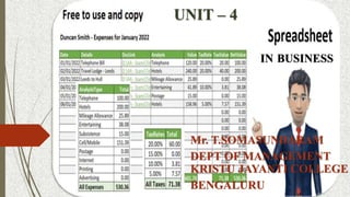
  • 1. Mr. T.SOMASUNDARAM DEPT OF MANAGEMENT KRISTU JAYANTI COLLEGE BENGALURU UNIT – 4 IN BUSINESS
  • 2. UNIT – 4 SPREADSHEET IN BUSINESS Introduction to Spreadsheet, Features of Spreadsheet, Cell reference, Format cells, Data Validation, Protecting Sheets, Data Analysis in Excel: Sort, Filter, Conditional Formatting, Preparing Charts, Pivot Table, What if Analysis (Goal seek, Scenario manager), Financial Functions: NPV, PMT, PV, FV, Rate, IRR, DB, SLN, SYD. Logical Functions: IF, AND, OR, Lookup Functions: V Lookup, H Lookup, Mathematical functions and text functions
  • 3. Introduction to Spreadsheet Microsoft Excel is spreadsheet software in the Microsoft Office Suite widely used to perform mathematical calculations. The data is spread in a tabular form consisting of rows and columns. It provides built-in features and tools such as formulas, functions and data analysis tools that make it easier to work with large amount of data. It allows to store, organize and analyse numerical and text data. A file of MS-Excel is called a Workbook and it contains multiple worksheets or spreadsheets primarily used to work with numbers and text. A worksheet is the grid of cells where you can type the data.
  • 4. Definition: “A Spreadsheet is a file that exists of cells in rows and columns and can help to arrange, calculate and sort data”. MS-Excel helps us to – Arrange data in an organized way. Perform calculations. Compare data through charts. Sort data for better analysis. Compare two workbooks side by side.
  • 5. Features of MS-Excel: Some of the main features of MS-Excel are – Excel provides support for multiple sheets within a workbook. It provides a standard grid, which may be scrolled and zoomed. Text, numeric or date values or formulas may be entered into selected cell through formula bar at the top of screen. A worksheet may be selected simply by tapping on it & can create or delete or rename existing worksheets. Cells may be formatted using format pages, specify font style, borders, text and background colours, size of cells and text alignment.
  • 6. Features of MS-Excel: Excel provides the ability to search worksheet for any phrase, number or other text, letting you easily scroll between search results. Excel supports a variety of functions used to perform basic calculations based on parameters set by user. Spreadsheets can be integrated for use with other software programs. (E.g.) Mail merge Professional looking graphs and charts can be created very quickly from a range of data which allows you to view the data pictorially. Easy to make changes and corrections to data on the worksheet.
  • 7. Spreadsheet (Excel) Elements or Terms 1. File Tab – it helps you to manage the Microsoft application and provide access to its options such as Open, New Save, As Print, etc. 2. Quick Access Toolbar – displays quick access to commonly used commands. 3. Ribbon – displays groups of related commands within tabs. Each tabs provides buttons for commands. 4. Tabs – it appears across the top of the Ribbon and contain groups of related commands. (E.g.) Home, Insert and Page Layout. 5. Title Bar – displays the name of the application file or document title. 6. Search Bar – advance search will help you find and perform tasks. 7. Name box – displays the active cell location. 8. Cell – intersection of a row and column, cells are always named with
  • 8. Spreadsheet (Excel) Elements or Terms 9. Formula Bar – displays the address of the active cell on the left edge and it also shows the current cell’s contents. 10. Status Bar – displays information about the current worksheet. 11. Zoom control – use to zoom the excel screen in or out by dragging the slider. 12. View Button or Option – displays worksheet view mode like normal layout view or page layout view or page break view. 13. Sheet Area – the area where you enter the data. 14. Row Bar – rows are numbered from 1 onwards and keeps on increasing as you keep entering data. 15. Column Bar – columns are numbered from A onwards and keeps on increasing as you keep entering data.
  • 10.
  • 13. Cell Reference Cell Referencing: The cell address in a formula is known as the cell reference. With the help of cell references, you can use the data in different parts of a worksheet. Types of cell referencing: 1. Relative Reference: When you create a formula, references to cell(s) are usually based on the position relative to the cell. When you copy or move a formula to other cells, the reference cell automatically changes.
  • 14. (E.g.) In the below figure, the formula in A3 cell is = A1 + A2. When you copy the formula from A3 cell to B3 cell, excel automatically changes the reference cell to match the location of cells. (i.e.) B3 cell is = B1 + B2.
  • 15. Cell Reference 2. Absolute Reference: Absolute reference is used when you do not want to change the address of the cell on copying the formula to another cell. For this purpose, you have to add the dollar symbol ($) before the column and the row number. (E.g.) In the below figure, enter the numbers you want to calculate in B2 cell and B3 cell. Create a simple formula = B2+B3 in B5 cell. To create an absolute reference in the formula, insert a $ symbol before the B (column reference) and 2 (row reference) in reference to B2, so new formula is =$B$2+B3.
  • 16.
  • 17. Copy and Paste the formula to another adjacent cell D5. The formula now includes absolute reference to B2, (=$B$2+D3)
  • 18. Cell Reference 3. Mixed Reference: It is a combination of Relative and Absolute reference. In this type of reference, either row or column has to remain fixed. (E.g.) In the below figure, enter the numbers you want to calculate in A1 cell and A2 cell. Create a simple formula = A1+A2 in A3 cell. To create a mixed reference in the formula, insert a $ symbol before the A (column reference) for A1 cell and 2 (row reference) in reference to A2 cell, so new formula is =$A1+A$2.
  • 19.
  • 20. Copy and Paste the formula to another adjacent cell B3. The formula now includes absolute reference to B3, (=$A1+B$2)
  • 21. Format Cells Once the data have entered into a worksheet, we need to format it in different ways like - Format Text in Bold or Italics Format Text as underlined Change the Font Style Change the Font Size Change the Text Colour Add a Border Add a fill colour Column Width Row height Insert / Delete Rows Insert / Delete Columns Wrap Text Merge Cells
  • 22. Data Validation Data Validation is an important task and to restrict data entry to certain range of dates, limit choices by using a list, entering only whole numbers, etc. It provides instructions to users and clear messages when invalid data is entered is also essential to make the data entry experience go smoothly.
  • 23. Protecting Sheets To prevent others users from accidentally or deliberately changing, moving or deleting data in a worksheet, we can lock the excel worksheet and then protect the sheet with a password. The two step process are – Step 1: Unlock any cells that needs to be editable. Step 2: Protect the worksheet & allow the users of this Worksheet to list, select the Elements what you want people to be able to change.
  • 24.
  • 25. Data Analysis in Excel Sorting or Data Sorting: Sorting or Data Sorting is a common spreadsheet task that allows you to easily reorder your data. The most common type of sorting is alphabetical ordering, which you can do in ascending or descending order. To Sort in Alphabetical Order: Select a cell in the column you want to sort. Click the Sort & Filter command in the Editing group on the Home tab. Select Sort A to Z. Now, the data in the spreadsheet will be organized alphabetically.
  • 27. Data Analysis in Excel To Sort in Numerical Order: Select a cell in the column you want to sort. Click the Sort & Filter command in the Editing group on the Home tab. Select Smallest to Largest. Now, the data in the spreadsheet will be organized numerically from the smallest to largest value.
  • 29. Data Analysis in Excel To Sort by Date or Time: Select a cell in the column you want to sort. Click the Sort & Filter command in the Editing group on the Home tab. Select Sort Oldest to Newest. Now, the data in the spreadsheet will be organized by date or time.
  • 30. Sort by date or time
  • 31. Data Analysis in Excel Filtering: Filtering is a convenient and reliable way to locate and manage spreadsheet data. This allows you to focus on specific spreadsheet entries. Filtered data can be copied, manipulated and printed without having to move it to a new spreadsheet. Data Filtering in Excel enables the user to work with a subset of data within the data list. When filter is created, only the records that contain the values specified are displayed. Other records in the data list are hidden temporarily.
  • 32. To Filter Data: Open the spreadsheet in which you want to filter data. Prepare your data for an Excel Auto filter. Select any cell within the range that you would like to filter. Select Filter Command in Sort & Filter group under Data tab. Drop down arrows will appear at the top of each column range. Click the drop-down arrow of the column containing the desired criteria to be filtered. To filter the data by criteria, click to clear the Select All check box and all other boxes will be cleared. Click to Select the check boxes of criteria that you want to appear in the filtered list. Click OK to filter the range by selected criteria.
  • 33.
  • 34.
  • 35.
  • 36. Data Analysis in Excel Conditional Formatting: A format, such as cell shading or font colour, that Excel automatically applies to cells if a specified condition is true. Conditional Formatting is a special formatting feature of excel that sets a cell’s format according to condition that you specify. Conditional Formatting allows you to present numeric data in different colours. (E.g.) you can shade data depending on whether the value is greater, equal to, or less than zero.
  • 37. Conditional Formatting: Open the spreadsheet and type the data in cells. Select the range of particular data. In Home Tab, under Styles group, Click Conditional Formatting command. A drop down list will be displayed. Click Highlight Cells Rules – Greater Than. Greater than dialog box will be appeared. Enter the value in any field (Greater or Less than or Equal to) and select colour fill field option from “with: drop down list”. Click OK. The final result of conditional formatting will appear.
  • 38.
  • 39.
  • 40. Data Analysis in Excel Preparing Charts: Charts (also known as graphs) are a visual representation of data in a worksheet. Charts allow you to present data entered into the worksheet in a visual format using a variety of graph types. Charts make it easy to see comparisons, patterns and trends in data. Components of a Chart: 1. Source Data - this is range of cells that make up a chart. 2. Title – this is the title of the chart.
  • 41. 3. Legend - this is the chart key, which describes what each colour on the chart represents. 4. Axis – this is vertical and horizontal parts of a chart. The vertical axis is often referred to as the Y axis, while the horizontal axis is referred to as the X axis. 5. Data Series – this is the actual charted values, which usually are rows or columns of the source data. 6. Value Axis – this is the axis that represents the values or units of the source data. 7. Category Axis – this is the axis identifying each data series.
  • 42. Types of Charts: 1. Area Chart: Area chart emphasizes the trend of each value over time. An area chart also shows the relationship of parts to a whole. 2. Column Chart: Column chart uses vertical bars or columns to represent data. They can work with many different types of data.
  • 43. 3. Bar Chart: Bar chart is similar to a column chart except these use horizontal instead of vertical bars. The bar chart shows variations in value over time. 4. Line Chart: Line chart shows trends and variations in data over time. Line chart displays a series of points, called data points, that are connected with lines and see whether values are increasing or decreasing over time.
  • 44. 5. Pie Chart: Pie Chart displays the contribution of each value to the total. Pie chart are very effective way to display information when you want to represent different parts of the whole or percentages of a total. In Pie Chart, each value is shown as a slice of the pie, so it is easy to see which values make up the percentage of a whole.
  • 45. To create Chart: First of all, enter the data into the worksheet and highlight all cell that will included in chart including column titles and row labels. Select the source data for the chart. Click the Insert tab. Select desired chart category. The chart will appear in the worksheet. To change chart types, Select the chart and Click the Design Tab. In Type group, click the Change Chart Type command. Change Chart type dialog box appears. Select the desired chart type, and then Click OK.
  • 46.
  • 47. Data Analysis in Excel Pivot Table: Pivot tables are interactive tables that allow the user to group and summarize large amounts of data in a concise, tabular format for easier reporting and analysis. They can sort, count and total the data, and are available in a variety of spreadsheet programs. Pivot table allows you to summarize your data more quickly and with more flexibility. Pivot tables are great way to summarize, analyze, explore and present your data and you can create them with just a few clicks.
  • 48. To create a Pivot Table: Select the Table or Cells, including column headers containing data you want to use. Click Insert Tab --- Tables group --- Pivot Table command. Select Pivot Table option from drop down list. Create Pivot table dialog box will appear. Make sure settings are correct, then Click OK. A blank Pivot Table will appear on left, Field list will appear on right side of worksheet. To Add Fields to Pivot Table – according to requirements, we have to decide which fields to add to Pivot Table. Each field is a column header from source data. To Change Row Labels – drag any existing field out of Row labers, and it will disappear.
  • 49.
  • 50.
  • 51.
  • 52.
  • 53.
  • 54. Data Analysis in Excel What if Analysis: It is a tool that enables you to find the input values needed to achieve a goal or objective. Goal Seek Feature: Goal seek feature allows you to change the data used in a formula in order to find out what results will be. To use Goal Seek, select the cell containing formula that will return the result you are seeking and then indicate the target value you want the formula to return and location of input value that Excel can change to reach the target.
  • 55. To use Goal Seek: Select the cell containing the formula that will return the result you are seeking. On the Data tab, Choose What-if Analysis ----- Goal seek in the Data Tools group. Goal Seek Dialog box will open. Cell is active cell when you open this dialog box, Set cell text box already contains the cell reference (E.g.) C1. Select the To Value text box and enter the goal. This is the value you want the formula in Set Cell box to reach. Select By changing cell text box and select cell that you want to change. Click OK and it displays Goal Seek status dialog box along with the results.
  • 56.
  • 57. Scenario Manager: The use of Scenario Manager in Excel allows you to have a certain set of inputs and outputs for a “Scenario”, and then lets you view different scenarios of outputs as the inputs change. This can help give people information to make decisions on their business based on different outcomes displayed by Scenario Manager. Excel’s Scenario Manager lets you create and save sets of different input values that produce different calculated results as named scenarios. The key to creating various scenarios for table is to identify various cells in data whose values can vary in each scenario.
  • 58. To use Scenario Manager: Open the spreadsheet containing the data for which you want to create scenario. On the Data tab of Ribbon, Choose What-If Analysis ----- Scenario Manager in the Data Tools group. The Scenario Manager dialog box appears. To create a Scenario, Click the Add button. Add Scenario dialog box appears. Type the name of scenario in Scenario name text box, specify the Changing Cells, Click OK. Excel displays the Scenario Values dialog box. Enter the values for each of changing cells in the text boxes. Click on Add button. Excel redisplays Add Scenario dialog box.
  • 59. To use Scenario Manager: Repeat the steps to enter the other scenarios. When you finish entering values for the final scenario, click OK instead of Add. Scenario manager dialog box makes another appearances, this time displaying the names of all scenarios in its Scenarios list box. To have Excel plug the changing values from any scenario into the table, click the scenario name in the Scenarios list box and then Click Show. Click the Close button when you are finished with the Scenario Manager.
  • 60.
  • 61.
  • 62.
  • 63.
  • 64. Financial Functions Financial functions calculate financial information, such as net present value and payments. (E.g.) Calculate monthly payments required to buy a car at a certain loan rate using the PMT function. Some of the commonly used financial functions are – 1. RATE: The RATE function is used to calculate the interest rate charged on a loan. 2. NPER: The NPER function is used to calculate the total number of periods (months, quarters, years) over which the loan or investment is to be paid.
  • 65. 3. PMT: The PMT function calculates the payment for a loan based on constant payments and a constant interest rate. It includes principal and interest but no other fees or taxes. 4. PV: The PV function calculates the present value of a loan or an investment, based on a constant interest rate. 5. FV: The FV function calculates the future value of an investment based on a constant interest rate. 6. NPV: The NPV function calculates the net present value of an investment using a discount rate and a series of future cash flows.
  • 66. 7. IRR: The IRR function returns the internal rate of return for a series of cash flows that occur at regular intervals. 8. DB: The DB function returns the depreciation value of an asset during a mentioned period by using fixed declining balance method. 9. SLN: The SLN function returns the straight-line depreciation of an asset for one period. 10. SYD: The SYD function returns the “sum of years” depreciation for an asset in a given period.
  • 68.
  • 71.
  • 74.
  • 77.
  • 79. Logical Functions Logical functions are used frequently for testing conditions and making decisions. Some of the commonly used logical functions are – 1. IF: The IF Function checks whether a condition is met or not. It returns one value if the condition is TRUE and another value if the condition is FALSE. (E.g.) Select Cell C1, enter the function =IF(A1>=33,”PASS”,”FAIL”) and Press ENTER.
  • 80. 2. AND: The AND Function returns TRUE if all conditions are true and returns FALSE if any of the conditions are false. (E.g.) Select Cell C4, enter the function =IF(AND(A4>=60,B4<100),”FIRST”,”SECOND”) and Press ENTER. Here AND function returns FALSE because the value in cell A4 is not greater than or equal to 60, though the value in cell B4 is less than 100. So second condition is true and first condition is false.
  • 81. 3. OR: The OR Function returns TRUE if any of the conditions are TRUE and returns FALSE if all conditions are false. (E.g.) Select Cell C8, enter the function =IF(OR(A8>=60,B8<100),”FIRST”,”SECOND”) and Press ENTER. Here ORD function returns TRUE because the value in cell B4 is less than 100, though the value in cell A4 is not greater than or equals to 60. So one of the two condition, one is true.
  • 82. Lookup Functions The lookup and reference functions help you to work with arrays of data, and are particularly useful when you need to cross reference between different data sets. Some of the commonly used lookup and reference functions are – 1. HLOOKUP: The HLOOKUP function looks up a supplied value in first row of a table and returns the corresponding value from another row. Syntax: HLOOKUP(lookup_value,table_array,row_index_num,[range_lookup]) Here,  Lookup_value – value that you want to search for, in the first row of the supplied data array (table).
  • 83. Lookup Functions  Table array – the data array or table, containing the data to be searched in the top row, and the return values in any other row.  Row_index_num – the row number, within the supplied table_array, that you want the corresponding value to be returned from.  [range_lookup] – an optional logical argument, which can be set to TRUE or FALSE, means: • TRUE – if function cannot find an exact match to the supplied lookup_value, it should use the closest match below the supplied value. • FALSE – if the function cannot find an exact match to the supplied lookup_value, it should return an error.
  • 84.
  • 85.  In this output table, HLOOKUP function searches through the top row of the table_array (A2-F2), to find a match for lookup_value (name Ed). When the name Ed is found, the function returns the corresponding value from 5th row of table_array.
  • 86. 2. VLOOKUP: The VLOOKUP function looks up a supplied value in first column of a table and returns the corresponding value from another column. Syntax: VLOOKUP(lookup_value,table_array,col_index_num,[range_lookup]) Here,  Lookup_value – value that you want to look up.  Table_array – the data array or table, containing the search values in the left hand columns and return values in another column.  Col_index_num – the column number, within supplied table_array, that you want to return a value from.  [range_lookup] – an optional logical argument that describes what the function should return in the event that it does not find an exact match to the lookup_value.
  • 87.  The [range_lookup] can be set to TRUE or FALSE, means: • TRUE – if function cannot find an exact match to the supplied lookup_value, it should use the closest match below the supplied value. • FALSE – if the function cannot find an exact match to the supplied lookup_value, it should return an error.
  • 88.
  • 89.  The above VLOOKUP function returns the price for “Cornflakes”, which is $3.50 In this output,  The lookup_value is the text string “Cornflakes”, which is located in cell I12.  The table_array is columns I-J of the spreadsheet.  The col_index_num is set to 2, to denote that the value returned should be taken from column 2 of the table_array.  The [range_lookup] argument is set to FALSE, to indicate that we only want a result to be returned if an exact match to the lookup_value is found.
  • 90. Mathematical Functions  Excel’s Mathematical functions can be used to perform common mathematical operations such as addition, multiplication and rounding numbers. Some of the commonly used mathematical functions are discussed below - 1. SUM – the SUM function adds together a supplied set of numbers and returns the sum of these values.  (E.g.) In spreadsheet SUM function is used to calculate the sum of numbers 5, 6, 7, 8 & 9.
  • 91. 2. PRODUCT – the PRODUCT function returns the product of a supplied set of numerical values.  (E.g.) In spreadsheet PRODUCT function is used to calculate the product of numbers 3, 6, 2, 8 & 5.
  • 92. 3. POWER – the POWER function calculates a given number, raised to a supplied power.  (E.g.) The following spreadsheet shows the use of POWER function -
  • 93. 4. SQRT – the SQRT function calculates the positive square root of a supplied number. If supplied number is negative, the SQRT function returns the #NUM! Error.  (E.g.) The following spreadsheet shows the use of SQRT function -
  • 94. 5. MOD – the MOD function returns the remainder of a division between two supplied numbers.  (E.g.) The following spreadsheet shows the use of MOD function -
  • 95. 6. ROUND – the ROUND function rounds a supplied number up or down, to a specified number of decimal places.  (E.g.) The following spreadsheet shows the use of ROUND function -
  • 96. Text Functions  Excel has many functions to offer when it comes to manipulating text or strings. Some of the commonly used text functions are discussed below - 1. LEFT – the LEFT function is used to extract the leftmost characters from a string. It returns a specified number of characters from the start of a supplied text string.
  • 97. 2. RIGHT – the RIGHT function is used to extract the rightmost characters from a string. It returns a specified number of characters from the end of a supplied text string.
  • 98. 3. MID – the MID function is used to extract a substring, starting in the middle of a string. It returns a specified number of characters from the middle of a supplied text string.
  • 99. 4. LEN – the LEN function is used to get the length of a string. It returns the length of a supplied text string.
  • 100. 5. FIND – the FIND function is used to find the position of a substring in a string. It returns the position of a specified character or sub-string within a supplied text string.
  • 101. 6. LOWER – the LOWER converts all characters in a supplied text string to lower case.
  • 102. 7. UPPER – the UPPER converts all characters in a supplied text string to upper case.