Top schools in delhi ncr

CHAPTER 2
Properties of Fluids
In this chapter we discuss a number of fundamental properties of fluids. An
understanding of these properties is essential for us to apply basic principles
of fluid mechanics to the solution of practical problems.
2.1 DISTINCTION BETWEEN A SOLID AND A FLUID
The molecules of a solid are usually closer together than those of a fluid. The
attractive forces between the molecules of a solid are so large that a solid tends
to retain its shape. This is not the case for a fluid, where the attractive forces be-tween
the molecules are smaller. An ideal elastic solid will deform under load
and, once the load is removed, will return to its original state. Some solids are
plastic. These deform under the action of a sufficient load and deformation con-tinues
as long as a load is applied, providing the material does not rupture. De-formation
ceases when the load is removed, but the plastic solid does not return
to its original state.
The intermolecular cohesive forces in a fluid are not great enough to hold
the various elements of the fluid together. Hence a fluid will flow under the ac-tion
of the slightest stress and flow will continue as long as the stress is present.
2.2 DISTINCTION BETWEEN A GAS AND A LIQUID
A fluid may be either a gas or a liquid. The molecules of a gas are much farther
apart than those of a liquid. Hence a gas is very compressible, and when all ex-ternal
pressure is removed, it tends to expand indefinitely. A gas is therefore in
equilibrium only when it is completely enclosed. A liquid is relatively incom-pressible,
and if all pressure, except that of its own vapor pressure, is removed,
the cohesion between molecules holds them together, so that the liquid does not
expand indefinitely. Therefore a liquid may have a free surface, i.e., a surface
from which all pressure is removed, except that of its own vapor.
A vapor is a gas whose temperature and pressure are such that it is very
near the liquid phase. Thus steam is considered a vapor because its state is
13

14 CHAPTER 2: Properties of Fluids
normally not far from that of water. A gas may be defined as a highly super-heated
vapor; that is, its state is far removed from the liquid phase. Thus air is
considered a gas because its state is normally very far from that of liquid air.
The volume of a gas or vapor is greatly affected by changes in pressure or
temperature or both. It is usually necessary, therefore, to take account of
changes in volume and temperature in dealing with gases or vapors. Whenever
significant temperature or phase changes are involved in dealing with vapors
and gases, the subject is largely dependent on heat phenomena (thermodynam-ics).
Thus fluid mechanics and thermodynamics are interrelated.
2.3 DENSITY, SPECIFICWEIGHT, SPECIFIC VOLUME,
AND SPECIFIC GRAVITY
The density r (rho),1 or more strictly, mass density, of a fluid is its mass per unit
volume, while the specific weight g (gamma) is its weight per unit volume. In the
British Gravitational (BG) system (Sec. 1.5) density r will be in slugs per cubic
foot (kg/m3 in SI units), which can also be expressed as units of lbsec2/ft4
(Ns2/m4 in SI units) (Sec. 1.5 and inside covers).
Specific weight g represents the force exerted by gravity on a unit volume
of fluid, and therefore must have the units of force per unit volume, such as
pounds per cubic foot (N/m3 in SI units).
Density and specific weight of a fluid are related as:
(2.1)
r
g
g or g rg
Since the physical equations are dimensionally homogeneous, the dimen-sions
of density are
Dimensions of r
In SI units
dimensions of g
dimensions of g
Dimensions of r

dimensions of g
dimensions of g
lb/ft3
ft/sec2

lbsec2
ft4
N/m3
m/s2
Ns2
m4
mass
volume
mass
volume

slugs
ft3
kg
m3
Note that density r is absolute, since it depends on mass, which is indepen-dent
of location. Specific weight g, on the other hand, is not absolute, since it de-pends
on the value of the gravitational acceleration g, which varies with loca-tion,
primarily latitude and elevation above mean sea level.
Densities and specific weights of fluids vary with temperature. Appendix A
provides commonly needed temperature variations of these quantities for water
1 The names of Greek letters are given in the List of Symbols on page xix.

2.3 Density, Specific Weight, Specific Volume, and Specific Gravity 15
and air. It also contains densities and specific weights of common gases at stan-dard
atmospheric pressure and temperature. We shall discuss the specific weight
of liquids further in Sec. 2.6.
Specific volume v is the volume occupied by a unit mass of fluid.2We com-monly
apply it to gases, and usually express it in cubic feet per slug (m3/kg in
SI units). Specific volume is the reciprocal of density. Thus
(2.2)
v
1
r
Specific gravity s of a liquid is the dimensionless ratio
sliquid
rliquid
rwater at standard temperature
Physicists use 4°C (39.2°F) as the standard, but engineers often use 60°F
(15.56°C). In the metric system the density of water at 4°C is 1.00 g/cm3 (or
1.00 g/mL),3 equivalent to 1000 kg/m3, and hence the specific gravity (which is
dimensionless) of a liquid has the same numerical value as its density expressed
in g/mL or Mg/m3. Appendix A contains information on specific gravities and
densities of various liquids at standard atmospheric pressure.
The specific gravity of a gas is the ratio of its density to that of either hy-drogen
or air at some specified temperature and pressure, but there is no gen-eral
agreement on these standards, and so we must explicitly state them in any
given case.
Since the density of a fluid varies with temperature, we must determine
and specify specific gravities at particular temperatures.
SAMPLE PROBLEM 2.1 The specific weight of water at ordinary pressure and
temperature is 62.4 lb/ft3. The specific gravity of mercury is 13.56. Compute the
density of water and the specific weight and density of mercury.
Solution
ANS
ANS
rwater
gwater
g
62.4 lb/ft3
32.2 ft/sec2 1.938 slugs/ft3
gmercury smercurygwater 13.56(62.4) 846 lb/ft3
rmercury smercuryrwater 13.56(1.938) 26.3 slugs/ft3 ANS
2 Note that in this book we use a “rounded” lower case v (vee), to help distinguish it
from a capital V and from the Greek n (nu).
3 One cubic centimeter (cm3) is equivalent to one milliliter (mL).

SAMPLE PROBLEM 2.2 The specific weight of water at ordinary pressure and
temperature is 9.81 kN/m3. The specific gravity of mercury is 13.56. Compute the
density of water and the specific weight and density of mercury.
Solution
ANS
ANS
rwater
9.81 kN/m3
9.81 m/s2 1.00 Mg/m3 1.00 g/mL
gmercury smercurygwater 13.56(9.81) 133.0 kN/m3
rmercury smercuryrwater 13.56(1.00) 13.56 Mg/m3 ANS
EXERCISES
2.3.1 If the specific weight of a liquid is 52 lb/ft3, what is its density?
2.3.2 If the specific weight of a liquid is 8.1 kN/m3, what is its density?
2.3.3 If the specific volume of a gas is 375 ft3/slug, what is its specific weight in lb/ft3?
2.3.4 If the specific volume of a gas is 0.70 m3/kg, what is its specific weight in N/m3?
2.3.5 A certain gas weighs 16.0 N/m3 at a certain temperature and pressure. What are
the values of its density, specific volume, and specific gravity relative to air
weighing 12.0 N/m3?
2.3.6 The specific weight of glycerin is 78.6 lb/ft3. Compute its density and specific
gravity. What is its specific weight in kN/m3?
2.3.7 If a certain gasoline weighs 43 lb/ft3, what are the values of its density, specific
volume, and specific gravity relative to water at 60°F? Use Appendix A.
2.4 COMPRESSIBLE AND INCOMPRESSIBLE FLUIDS
Fluid mechanics deals with both incompressible and compressible fluids, that
is, with liquids and gases of either constant or variable density. Although there
is no such thing in reality as an incompressible fluid, we use this term where
the change in density with pressure is so small as to be negligible. This is usually
the case with liquids. We may also consider gases to be incompressible when the
pressure variation is small compared with the absolute pressure.
Ordinarily we consider liquids to be incompressible fluids, yet sound
waves, which are really pressure waves, travel through them. This is evidence of
the elasticity of liquids. In problems involving water hammer (Sec. 12.6) we
must consider the compressibility of the liquid.
The flow of air in a ventilating system is a case where we may treat a gas as
incompressible, for the pressure variation is so small that the change in density
is of no importance. But for a gas or steam flowing at high velocity through a
long pipeline, the drop in pressure may be so great that we cannot ignore the
change in density. For an airplane flying at speeds below 250 mph (100 m/s), we

2.5 Compressibility of Liquids 17
may consider the air to be of constant density. But as an object moving through
the air approaches the velocity of sound, which is of the order of 760 mph
(1200 km/h) depending on temperature, the pressure and density of the air ad-jacent
to the body become materially different from those of the air at some dis-tance
away, and we must then treat the air as a compressible fluid (Chap. 13).
2.5 COMPRESSIBILITY OF LIQUIDS
The compressibility (change in volume due to change in pressure) of a liquid is
inversely proportional to its volume modulus of elasticity, also known as the
bulk modulus. This modulus is defined as
Ev v
dp
dv
a v
dvb˛dp
where v specific volume and p pressure. As vdv is a dimensionless ratio,
the units of Ev and p are identical. The bulk modulus is analogous to the modu-lus
of elasticity for solids; however, for fluids it is defined on a volume basis
rather than in terms of the familiar one-dimensional stress–strain relation for
solid bodies.
In most engineering problems, the bulk modulus at or near atmospheric
pressure is the one of interest. The bulk modulus is a property of the fluid and
for liquids is a function of temperature and pressure. A few values of the bulk
modulus for water are given in Table 2.1. At any temperature we see that the
value of Ev increases continuously with pressure, but at any one pressure the
value of Ev is a maximum at about 120°F (50°C). Thus water has a minimum
compressibility at about 120°F (50°C).
Note that we often specify applied pressures, such as those in Table 2.1, in
absolute terms, because atmospheric pressure varies. The units psia or kN/m2
abs indicate absolute pressure, which is the actual pressure on the fluid, relative
TABLE 2.1 Bulk modulus of water Ev, psia
Temperature, °F
Pressure, psia 32° 68° 120° 200° 300°
15 293,000 320,000 333,000 308,000
1,500 300,000 330,000 342,000 319,000 248,000
4,500 317,000 348,000 362,000 338,000 271,000
15,000 380,000 410,000 426,000 405,000 350,000
a These values can be transformed to meganewtons per square meter by multiplying
them by 0.006895. The values in the first line are for conditions close to normal
atmospheric pressure; for a more complete set of values at normal atmospheric
pressure, see Table A.1 in Appendix A. The five temperatures are equal to 0, 20, 48.9,
93.3, and 148.9°C, respectively.

to absolute zero. The standard atmospheric pressure at sea level is about
14.7 psia or 101.3 kN/m2 abs (1013 mb abs) (see Sec. 2.9 and Table A.3). Bars
and millibars were previously used in metric systems to express pressure; 1 mb
100 N/m2. We measure most pressures relative to the atmosphere, and call
them gage pressures. This is explained more fully in Sec. 3.4.
The volume modulus of mild steel is about 26,000,000 psi (170000 MN/m2).
Taking a typical value for the volume modulus of cold water to be 320,000 psi
(2200 MN/m2), we see that water is about 80 times as compressible as steel. The
compressibility of liquids covers a wide range. Mercury, for example, is approx-imately
8% as compressible as water, while the compressibility of nitric acid is
nearly six times greater than that of water.
In Table 2.1 we see that at any one temperature the bulk modulus of water
does not vary a great deal for a moderate range in pressure. By rearranging the
definition of Ev, as an approximation we may use for the case of a fixed mass of
liquid at constant temperature
(2.3a)
or (2.3b)
where Ev is the mean value of the modulus for the pressure range and the sub-scripts
1 and 2 refer to the before and after conditions.
Assuming Ev to have a value of 320,000 psi, we see that increasing the pres-sure
of water by 1000 psi will compress it only or 0.3%, of its original volume.
Therefore we find that the usual assumption regarding water as being incom-pressible
is justified.
1
320,
v2 v1
v1

p2 p1
Ev
Dv
v

Dp
Ev
SAMPLE PROBLEM 2.3 At a depth of 8 km in the ocean the pressure is
81.8 MPa. Assume that the specific weight of seawater at the surface is
10.05 kN/m3 and that the average volume modulus is 2.34 109 N/m2 for that
pressure range. (a) What will be the change in specific volume between that at the
surface and at that depth? (b) What will be the specific volume at that depth?
(c) What will be the specific weight at that depth?
Solution
1
8 km Sea water
2
1 10.05 kN/m3
p2 81.8 MPa

2.6 Specific Weight of Liquids 19
(a) Eq. (2.2): v1 1r1 gg1 9.8110050 0.000976 m3/kg
Eq. (2.3a):

Dv 0.000 976(81.8106 0)(2.34109)
ANS
34.1106 m3/kg
v2 v1 Dv 0.000 942 m3/kg
(b) Eq. (2.3b): ANS
(c) g2 gv2 9.810.000942 10410 N/m3 ANS
EXERCISES
2.5.1 To two significant figures what is the bulk modulus of water in MN/m2 at 50°C
under a pressure of 30 MN/m2? Use Table 2.1.
2.5.2 At normal atmospheric conditions, approximately what pressure in psi must be
applied to water to reduce its volume by 2%? Use Table 2.1.
2.5.3 Water in a hydraulic press is subjected to a pressure of 4500 psia at 68°F. If the
initial pressure is 15 psia, approximately what will be the percentage decrease in
specific volume? Use Table 2.1.
2.5.4 At normal atmospheric conditions, approximately what pressure in MPa must be
applied to water to reduce its volume by 3%?
2.5.5 A rigid cylinder, inside diameter 15 mm, contains a column of water 500 mm long.
What will the column length be if a force of 2 kN is applied to its end by a
frictionless plunger? Assume no leakage.
2 kN
Rigid Water L2
L1
500 mm
Figure X2.5.5
2.6 SPECIFICWEIGHT OF LIQUIDS
The specific weights g of some common liquids at 68°F (20°C) and standard sea-level
atmospheric pressure4 with g 32.2 ft/sec2 (9.81 m/s2) are given in Table
2.2. The specific weight of a liquid varies only slightly with pressure, depending
on the bulk modulus of the liquid (Sec. 2.5); it also depends on temperature,
and the variation may be considerable. Since specific weight g is equal to rg, the
4 See Secs. 2.9 and 3.5.
Water

specific weight of a fluid depends on the local value of the acceleration of gravity
in addition to the variations with temperature and pressure. The variation of the
specific weight of water with temperature and pressure, where g 32.2
ft/sec2
(9.81 m/s2), is shown in Fig. 2.1. The presence of dissolved air, salts in solution,
and suspended matter will increase these values a very slight amount. Ordinarily
TABLE 2.2 Specific weights g of common liquids at
68°F (20°C), 14.7 psia (1013 mb abs) with g 32.2
ft/sec2 (9.81 m/s2)
lb/ft3 kN/m3
Carbon tetrachloride 99.4 15.6
Ethyl alcohol 49.3 7.76
Gasoline 42 6.6
Glycerin 78.7 12.3
Kerosene 50 7.9
Motor oil 54 8.5
Seawater 63.9 10.03
Water 62.3 9.79
63.2
63.0
62.8
62.6
62.4
62.2
62.0
61.8
Specific weight , lb/ft3
Specific weight , kN/m3
61.6
61.4
61.2
61.0
60.8
60.6
0 10 20 30 40 50 60 70 80
30 50
Temperature, C
Atmospheric pressure, 14.7 psia (101.3 kPa abs)
70 90 110
Temperature, F
130 150 170
9.90
9.85
9.80
9.75
9.70
9.65
9.60
9.55
2000 psia (13.79 MPa abs)
1000 psia (6.89 MPa abs)
Figure 2.1
Specific weight g of pure water as a function of temperature and pressure for the
condition where g 32.2 ft/sec2 (9.81 m/s2).

we assume ocean water to weigh 64.0 lb/ft3 (10.1 kN/m3). Unless otherwise
specified or implied by a given temperature, the value to use for water in the
problems in this book is g 62.4
lb/ft3 (9.81 kN/m3). Under extreme conditions
the specific weight of water is quite different. For example, at 500°F (260°C) and
6000 psi (42 MN/m2) the specific weight of water is 51 lb/ft3 (8.0 kN/m3).
2.6 Specific Weight of Liquids 21
SAMPLE PROBLEM 2.4 A vessel contains 85 L of water at 10°C and
atmospheric pressure. If the water is heated to 70°C, what will be the percentage
change in its volume? What weight of water must be removed to maintain the
volume at its original value? Use Appendix A.
Solution
Volume,
Table A.1:
10C 70C
patm
V10 85 L V70
V10 85 L 0.085 m3
V
g10 9.804 kN/m3, g70 9.589 kN/m3
Weight of water,
W gV g10V10 g70V70
9.804(0.085) kN 9.589 V70; V70 0.086 91 m3
DV V70 V10 0.086 91 0.085 00 0.001 906 m3 at g70
DVV10 0.001 9060.085 2.24% increase
WaDV
V70 b g70 DV
EXERCISES
2.6.1 Use Fig. 2.1 to find the approximate specific weight of water in lb/ft3 under the
following conditions: (a) at a temperature of 60°C under 101.3 kPa abs pressure;
(b) at 60°C under a pressure of 13.79 MPa abs.
2.6.2 Use Fig. 2.1 to find the approximate specific weight of water in kN/m3 under the
following conditions: (a) at a temperature of 160°F under normal atmospheric
pressure; (b) at 160°F under a pressure of 2000 psia.
i.e.,
ANS
Must remove (at g70):
(9589 N/m3)(0.001 906 m3) 18.27 N ANS

2.6.3 A vessel contains 5.0 ft3 of water at 40°F and atmospheric pressure. If the water is
heated to 80°F, what will be the percentage change in its volume? What weight
of water must be removed to maintain the volume at its original value? Use
Appendix A.
2.6.4 A cylindrical tank (diameter 8.00 m and depth 5.00 m) contains water at
15°C and is brimful. If the water is heated to 60°C, how much water will spill over
the edge of the tank? Assume the tank does not expand with the change in
temperature. Use Appendix A.
2.7 PROPERTY RELATIONS FOR PERFECT GASES
The various properties of a gas, listed below, are related to one another (see,
e.g., Appendix A, Tables A.2 and A.5). They differ for each gas. When the con-ditions
of most real gases are far removed from the liquid phase, these relations
closely approximate those of hypothetical perfect gases. Perfect gases, are here
(and often) defined to have constant specific heats5 and to obey the perfect-gas
law,
(2.4)
p
r
pv RT
where p absolute pressure (Sec. 3.4)
r density (mass per unit volume)
specific volume (volume per unit mass, 1r)
v
R
a gas constant, the value of which depends upon the particular gas
T
absolute temperature in degrees Rankine or Kelvin6
For air, the value of R is 1715 ftlb/(slug°R) or 287 Nm/(kgK) (Appendix A,
Table A.5); making use of the definitions of a slug and a newton (Sec. 1.5), these
units are sometimes given as ft2/(sec2°R) and m2/(s2K), respectively. Since
Eq. (2.4) can also be written
(2.5)
g
gp
RT
g rg,
from which the specific weight of any gas at any temperature and pressure can
be computed if R and g are known. Because Eqs. (2.4) and (2.5) relate the vari-ous
gas properties at a particular state, they are known as equations of state and
as property relations.
In this book we shall assume that all gases are perfect. Perfect gases are
sometimes also called ideal gases. Do not confuse a perfect (ideal) gas with an
ideal fluid (Sec. 2.10).
5 Specific heat and other thermodynamic properties of gases are discussed in Sec. 13.1.
6 Absolute temperature is measured above absolute zero. This occurs on the
Fahrenheit scale at 459.67°F (0° Rankine) and on the Celsius scale at 273.15°C
(0 Kelvin). Except for low-temperature work, these values are usually taken as 460°F
and 273°C. Remember that no degree symbol is used with Kelvin.

2.7 Property Relations for Perfect Gases 23
Avogadro’s law states that all gases at the same temperature and pressure
under the action of a given value of g have the same number of molecules
per unit of volume, from which it follows that the specific weight of a gas7 is
proportional to its molar mass. Thus, if M denotes molar mass (formerly called
molecular weight), g2g1 M2M1 and, from Eq. (2.5), g2g1 R1R2
for the
same temperature, pressure, and value of g. Hence for a perfect gas
M1R1 M2R2 constant R0
R0 is known as the universal gas constant, and has a value of 49,709 ftlb/
(slug-mol°R) or 8312 Nm/(kg-molK). Rewriting the preceding equation in the
form
R
R0
M
enables us to obtain any gas constant R required for Eq. (2.4) or (2.5).
For real (nonperfect) gases, the specific heats may vary over large temper-ature
ranges, and the right-hand side of Eq. (2.4) is replaced by zRT, so that
R0 MzR,
where z is a compressibility factor that varies with pressure and tem-perature.
Values of z and R are given in thermodynamics texts and in hand-books.
However, for normally encountered monatomic and diatomic gases, z
varies from unity by less than 3%, so the perfect-gas idealizations yield good ap-proximations,
and Eqs. (2.4) and (2.5) will give good results.
When various gases exist as a mixture, as in air, Dalton’s law of partial
pressures states that each gas exerts its own pressure as if the other(s) were not
present. Hence it is the partial pressure of each that we must use in Eqs. (2.4)
and (2.5) (see Sample Prob. 2.5). Water vapor as it naturally occurs in the
atmosphere has a low partial pressure, so we may treat it as a perfect gas
with R 49,70918 2760
ftlb/(slug°R) [462 Nm/(kgK)]. But for steam at
higher pressures this value is not applicable.
As we increase the pressure and simultaneously lower the temperature, a
gas becomes a vapor, and as gases depart more and more from the gas phase and
approach the liquid phase, the property relations become much more compli-cated
than Eq (2.4), and we must then obtain specific weight and other proper-ties
from vapor tables or charts. Such tables and charts exist for steam, ammo-nia,
sulfur dioxide, freon, and other vapors in common engineering use.
Another fundamental equation for a perfect gas is
(2.6a)
n constant
pvn p1v1
p
p1
r1bn
ar
constant
or (2.6b)
v ( 1r)
where p is absolute pressure, is specific volume, r is density, and n may
have any nonnegative value from zero to infinity, depending on the process to
7 The specific weight of air (molar mass 29.0) at 68°F (20°C) and 14.7 psia (1013 mb
abs) with g 32.2 ft/sec2 (9.81 m/s2) is 0.0752 lb/ft3 (11.82 N/m3).

which the gas is subjected. Since this equation describes the change of the gas
properties from one state to another for a particular process, we call it a process
equation. If the process of change is at a constant temperature (isothermal),
If there is no heat transfer to or from the gas, the process is adiabatic. A
frictionless (and reversible) adiabatic process is an isentropic process, for which
we denote n by k, where , the ratio of specific heat at constant pressure
to that at constant volume.8 This specific heat ratio k is also called the adiabatic
exponent. For expansion with friction n is less than k, and for compression with
friction n is greater than k. Values for k are given in Appendix A, Table A.5, and
in thermodynamics texts and handbooks. For air and diatomic gases at usual
temperatures, we can take k as 1.4.
By combining Eqs. (2.4) and (2.6), we can obtain other useful relations
such as
(2.7)
T2
T1
v2bn1
av1
r1bn1
ar2
p1b(n1)n
ap2
k cpcv
n 1.
SAMPLE PROBLEM 2.5 If an artificial atmosphere consists of 20% oxygen and
80% nitrogen by volume, at 14.7 psia and 60°F, what are (a) the specific weight
and partial pressure of the oxygen and (b) the specific weight of the mixture?
Solution
Table A.5:
Eq. (2.5): 100% O2:
R (oxygen) 1554 ft2/(sec2°R),
R (nitrogen) 1773 ft2/(sec2°R)
32.2(14.7144)
1554(460 60)
32.2(14.7144)
0.0843 lb/ft3
0.0739 lb/ft3
g
Eq. (2.5): 100% N2:
g
1773(520)
(a) Each ft3 of mixture contains 0.2 ft3 of O2 and 0.8 ft3 of N2.
So for 20% O2, g 0.20(0.0843) 0.016 87 lb/ft3
ANS
From Eq. (2.5), for 20% O2,
ANS
p
gRT
g
0.016 87(1554)520
32.2
423 lb/ft2 abs 2.94 psia
Note that this 20%(14.7 psia).
(b) For 80% N2,
g 0.80(0.0739) 0.0591 lb/ft3.
Mixture: g 0.016 87 0.0591 0.0760 lb/ft3 ANS
8 Specific heat and other thermodynamic properties of gases are discussed in Sec. 13.1.

2.8 Compressibility of Perfect Gases 25
EXERCISES
2.7.1 A gas at 60°C under a pressure of 10000 mb abs has a specific weight of 99 N/m3.
What is the value of R for the gas? What gas might this be? Refer to Appendix A,
Table A.5.
2.7.2 A hydrogen-filled balloon of the type used in cosmic-ray studies is to be
expanded to its full size, which is a 100-ft-diameter sphere, without stress in
the wall at an altitude of 150,000 ft. If the pressure and temperature at this
altitude are 0.14 psia and 67°F respectively, find the volume of hydrogen at
14.7 psia and 60°F that should be added on the ground. Neglect the balloon’s
weight.
2.7.3 Calculate the density, specific weight, and specific volume of air at 120°F and
50 psia.
2.7.4 Calculate the density, specific weight, and specific volume of air at 50°C and
3400 mb abs.
2.7.5 If natural gas has a specific gravity of 0.6 relative to air at 14.7 psia and 68°F,
what are its specific weight and specific volume at that same pressure and
temperature. What is the value of R for the gas? Solve without using
Table A.2.
2.7.6 Given that a sample of dry air at 40°F and 14.7 psia contains 21% oxygen and
78% nitrogen by volume. What is the partial pressure (psia) and specific weight
of each gas?
2.7.7 Prove that Eq. (2.7) follows from Eqs. (2.4) and (2.6).
2.8 COMPRESSIBILITY OF PERFECT GASES
npvn1 dv vn
dp 0.
Differentiating Eq. (2.6) gives Inserting the value of dp
from this into from Sec. 2.5 yields
(2.8)
Ev np
Ev p,
Ev (vdv) dp
So for an isothermal process of a gas and for an isentropic process
.
Ev kp
Thus, at a pressure of 15 psia, the isothermal modulus of elasticity for a gas
is 15 psi, and for air in an isentropic process it is 1.4(15 psi) 21 psi. Assuming
from Table 2.1 a typical value of the modulus of elasticity of cold water to be
320,000 psi, we see that air at 15 psia is 320,00015 21,000 times as compress-ible
as cold water isothermally, or 320,00021 15,000 times as compressible
isentropically. This emphasizes the great difference between the compressibility
of normal atmospheric air and that of water.

SAMPLE PROBLEM 2.6 (a) Calculate the density, specific weight, and specific
volume of oxygen at 100°F and 15 psia (pounds per square inch absolute; see
Sec. 2.7). (b) What would be the temperature and pressure of this gas if we
compressed it isentropically to 40% of its original volume? (c) If the process
described in (b) had been isothermal, what would the temperature and pressure
have been?
Solution
n k 1.4 n 1
0.4V
0.4V
T2, p2 T2 100F, p2
V
Table A.5 for oxygen (O2): Molar mass
M 32.0, k 1.40
(a) Sec. 2.7: (as in Table A.5)
From Eq. (2.4):
ANS
0.002 48 slug/ft3
g 32.2 g rg 0.002 48(32.2) 0.0800 lb/ft3
With ft/sec2, ANS
1
r
1
403 ft3/slug
Eq. (2.2): ANS
v
(b) Isentropic compression:
Eq. (2.6) with

0.002 48
v2 40%v1 0.4(403) 161.1 ft3/slug
n k: pvk (15144)(403)1.4 (p2144)(161.1)1.4
psia ANS
From Eq. (2.4):
p2 54.1
p2 54.1144 psia rRT 0.006 21(1553)(460 T2)
ANS
(c) Isothermal compression: 100°F ANS
pv constant:
(15144)(403) (p2144)(0.4403)
p2 37.5 psia ANS
T2 T1
T2 348°F
r2 1v2 0.006 21 slug/ft3
r
p
RT

15144 lb/ft2
[1553 ftlb/(slug°R)][(460 100)°R]
R
R0
M

49,709
32.0
1553 ftlb/(slug°R)
100F, 15 psia
(a) (b) (c)

2.9 Standard Atmosphere 27
SAMPLE PROBLEM 2.7 Calculate the density, specific weight, and specific
volume of chlorine gas at 25°C and pressure of 600 kN/m2 abs (kilonewtons per
square meter absolute; see Sec. 2.7). Given the molar mass of chlorine
(Cl2) 71.
Solution
Sec. 2.7:
From Eq. (2.4):
117.1 Nm/(kgK)
600 000 N/m2

8312
71
[117.1 Nm/(kgK)][(273 25)K]
ANS
R0
M

17.20 kg/m3
R
r
p
RT
g 9.81 m/s2, g rg 17.20(9.81) 168.7 N/m3
With ANS
1
r
1
17.20
0.0581 m3/kg
Eq. (2.2): v
ANS
EXERCISES
2.8.1 Methane at 22 psia is compressed isothermally, and nitrogen at 16 psia is
compressed isentropically. What is the modulus of elasticity of each gas? Which
is the more compressible?
2.8.2 Methane at 140 kPa abs is compressed isothermally, and nitrogen at 100 kPa abs
is compressed isentropically. What is the modulus of elasticity of each gas? Which
is the more compressible?
2.8.3 (a) If 10 m3 of nitrogen at 30°C and 125 kPa are expanded isothermally to 25 m3,
what is the resulting pressure? (b) What would the pressure and temperature
have been if the process had been isentropic? The adiabatic exponent k for
nitrogen is 1.40.
2.8.4 Helium at 25 psia and 65°F is isentropically compressed to one-fifth of its original
volume. What is its final pressure?
2.9 STANDARD ATMOSPHERE
Standard atmospheres were first adopted in the 1920s in the United States and
in Europe to satisfy a need for standardization of aircraft instruments and air-craft
performance. As knowledge of the atmosphere increased, and man’s activ-ities
in it rose to ever greater altitudes, such standards have been frequently ex-tended
and improved.
The International Civil Aviation Organization adopted its latest ICAO
Standard Atmosphere in 1964, which extends up to 32 km (105,000 ft). The
International Standards Organization adopted an ISO Standard Atmosphere to

50 km (164,000 ft) in 1973, which incorporates the ICAO standard. The United
States has adopted the U.S. Standard Atmosphere, last revised in 1976. This in-corporates
the ICAO and ISO standards, and extends to at least 86 km
(282,000 ft or 53.4 mi); for some quantities it extends as far as 1000 km (621 mi).
Figure 2.2 graphically presents variations of temperature and pressure in
the U.S. Standard Atmosphere. In the lowest 11.02 km (36,200 ft), called the
troposphere, the temperature decreases rapidly and linearly at a lapse rate of
6.489°C/km (3.560°F1000 ft). In the next layer, called the stratosphere,
about 9 km (30,000 ft) thick, the temperature remains constant at 56.5°C
(69.7°F). Next, in the mesosphere, it increases, first slowly and then more
rapidly, to a maximum of 2.5°C (27.5°F) at an altitude around 50 km (165,000 ft
or 31 mi). Above this, in the upper part of the mesosphere known as the iono-sphere,
the temperature again decreases.
The standard absolute pressure9 behaves very differently from temperature
(Fig. 2.2), decreasing quite rapidly and smoothly to almost zero at an altitude of
9 Absolute pressure is discussed in Secs. 2.7 and 3.4.
Temperature, F
100 50 0 50
86.28C, 123.30F
86.000 km
90
80
70
60
50
40
Altitude, km
Altitude, 1000 ft
30
20
58.5C at 71.802 km
100 80 60 40
20 0 20
Temperature, C
10
0
51.413 km 2.5C,
56.5C, 69.7F
6.489C/km
3.560F/1000 ft
Absolute pressure, psia
0 5 10 15 20
Mesosphere
Ionosphere
0.868 kPa at 32.162 km
Mesosphere
Stratosphere
Troposphere
101.325 kPa
14.696 psia
15C,
59F
47.350 km
ISO limit
ICAO limit 44.5C at 32.162 km
20.063 km
11.019 km
0 50 100 150
Absolute pressure, kPa
300
250
200
150
100
50
0
27.5F
Figure 2.2
The U.S. Standard Atmosphere, temperature, and pressure distributions.

30 km (98,000 ft). The pressure profile was computed from the standard temper-atures
using methods of fluid statics (Sec. 3.2). The representation of the stan-dard
temperature profile by a number of linear functions of elevation (Fig. 2.2)
greatly facilitates such computations (see Sample Prob. 3.1d).
Temperature, pressure, and other variables from the ICAO Standard At-mosphere,
including density and viscosity, are tabulated together with gravita-tional
acceleration out to 30 km and 100,000 ft in Appendix A, Table A.3. Engi-neers
generally use such data in design calculations where the performance of
high-altitude aircraft is of interest. The standard atmosphere serves as a good
approximation of conditions in the atmosphere; of course the actual conditions
vary somewhat with the weather, the seasons, and the latitude.
2.10 IDEAL FLUID
An ideal fluid is usually defined as a fluid in which there is no friction; it is
inviscid (its viscosity is zero). Thus the internal forces at any section within it
are always normal to the section, even during motion. So these forces are
purely pressure forces. Although such a fluid does not exist in reality, many flu-ids
approximate frictionless flow at sufficient distances from solid boundaries,
and so we can often conveniently analyze their behaviors by assuming an ideal
fluid. As noted in Sec. 2.7, take care to not confuse an ideal fluid with a perfect
(ideal) gas.
In a real fluid, either liquid or gas, tangential or shearing forces always de-velop
whenever there is motion relative to a body, thus creating fluid friction,
because these forces oppose the motion of one particle past another. These fric-tion
forces give rise to a fluid property called viscosity.
2.11 VISCOSITY
The viscosity of a fluid is a measure of its resistance to shear or angular defor-mation.
Motor oil, for example, has high viscosity and resistance to shear, is co-hesive,
and feels “sticky,” whereas gasoline has low viscosity. The friction forces
in flowing fluid result from the cohesion and momentum interchange between
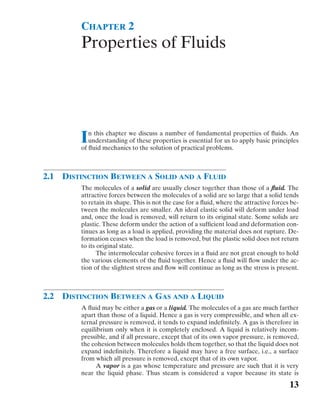
molecules. Figure 2.3 indicates how the viscosities of typical fluids depend on
temperature. As the temperature increases, the viscosities of all liquids decrease,
while the viscosities of all gases increase. This is because the force of cohesion,
which diminishes with temperature, predominates with liquids, while with gases
the predominating factor is the interchange of molecules between the layers of
different velocities. Thus a rapidly-moving gas molecule shifting into a slower-moving
layer tends to speed up the latter. And a slow-moving molecule entering
a faster-moving layer tends to slow down the faster-moving layer. This molecu-lar
interchange sets up a shear, or produces a friction force between adjacent
layers. At higher temperatures molecular activity increases, so causing the vis-cosity
of gases to increase with temperature.
2.11 Viscosity 29

Liquids
Gases
Temperature
Viscosity
(absolute and kinematic)
Figure 2.3
Trends in viscosity variation with temperature.
Figures A.1 and A.2 in Appendix A graphically present numerical values
of absolute and kinematic viscosities for a variety of liquids and gases, and show
how they vary with temperature.
Consider the classic case of two parallel plates (Fig. 2.4), sufficiently large
that we can neglect edge conditions, a small distance Y apart, with fluid filling
the space between. The lower plate is stationary, while the upper one moves par-allel
to it with a velocity U due to a force F corresponding to some area A of the
moving plate.
At boundaries, particles of fluid adhere to the walls, and so their velocities
are zero relative to the wall. This so-called no-slip condition occurs with all vis-cous
fluids. Thus in Fig. 2.4 the fluid velocities must be U where in contact with
the plate at the upper boundary and zero at the lower boundary. We call the
form of the velocity variation with distance between these two extremes, as de-picted
in Fig. 2.4, a velocity profile. If the separation distance Y is not too great,
if the velocity U is not too high, and if there is no net flow of fluid through the
space, the velocity profile will be linear, as in Fig. 2.4a. If, in addition, there is a
small amount of bulk fluid transport between the plates, as could result from
pressure-fed lubrication for example, the velocity profile becomes the sum of
F, U
U
y
Y
u
dy
Velocity
profile
du
F, U
U
y
u
Velocity
profile
Slope
Y du
dy
(a) Linear (no bulk flow) (b) Curved (bulk flow to the right)
Figure 2.4
Velocity profiles.

2.11 Viscosity 31
the previous linear profile plus a parabolic profile (Fig. 2.4b); the parabolic
additions to (or subtractions from) the linear profile are zero at the walls (plates)
and maximum at the centerline. The behavior of the fluid is much as if it con-sisted
of a series of thin layers, each of which slips a little relative to the next.
For a large class of fluids under the conditions of Fig. 2.4a, experiments
have shown that
F
AU
Y
We see from similar triangles that we can replace UY by the velocity gradient
dudy m
. If we now introduce a constant of proportionality (mu), we can express
t
the shearing stress (tau) between any two thin sheets of fluid by
(2.9)
t
F
A
m
U
Y
m
du
dy
We call Eq. (2.9) Newton’s equation of viscosity, since Sir Isaac Newton
(1642–1727) first suggested it. Although better known for his formulation of the
fundamental laws of motion and gravity and for the development of differential
calculus, Newton, an English mathematician and natural philosopher, also made
many pioneering studies in fluid mechanics. In transposed form, Eq. (2.9) de-fines
the proportionality constant
(2.10)
m
t
dudy
known as the coefficient of viscosity, the absolute viscosity, the dynamic vis-cosity
(since it involves force), or simply the viscosity of the fluid. We shall use
“absolute viscosity” to help differentiate it from another viscosity that we will
discuss shortly.
We noted in Sec. 2.1 that the distinction between a solid and a fluid lies in
the manner in which each can resist shearing stresses. We will clarify a further
distinction among various kinds of fluids and solids by referring to Fig. 2.5. In
Non-Newtonian fluid
t shear stress
Elastic solid
Ideal fluid
Ideal plastic
Newtonian fluid
Figure 2.5 du/dy

the case of a solid, shear stress depends on the magnitude of the deformation;
but Eq. (2.9) shows that in many fluids the shear stress is proportional to the time
rate of (angular) deformation.
A fluid for which the constant of proportionality (i.e., the absolute viscos-ity)
does not change with rate of deformation is called a Newtonian fluid, and
this plots as a straight line in Fig. 2.5. The slope of this line is the absolute vis-cosity,
m. The ideal fluid, with no viscosity (Sec. 2.10), falls on the horizontal axis,
while the true elastic solid plots along the vertical axis. A plastic that sustains
a certain amount of stress before suffering a plastic flow corresponds to a
straight line intersecting the vertical axis at the yield stress. There are certain
non-Newtonian fluids10 in which m varies with the rate of deformation. These
are relatively uncommon in engineering usage, so we will restrict the remainder
of this text to the common fluids that under normal conditions obey Newton’s
equation of viscosity.
In a journal bearing, lubricating fluid fills the small annular space between
a shaft and its surrounding support. This fluid layer is very similar to the layer
between the two parallel plates, except it is curved. There is another more sub-tle
difference, however. For coaxial cylinders (Fig. 2.6) with constant rotative
speed v (omega), the resisting and driving torques are equal. But because the
radii at the inner and outer walls are different, it follows that the shear stresses
10 Typical non-Newtonian fluids include paints, printer’s ink, gels and emulsions,
sludges and slurries, and certain plastics. An excellent treatment of the subject is given
by W. L. Wilkinson in NonNewtonian Fluids, Pergamon Press, New York, 1960.
U1 r1
Tr
Td
r1
r2
0

Y
(a)
U2 r2
Td
Tr

0
r1
r2
(b)
Figure 2.6
Velocity profile, rotating coaxial cylinders with gap completely filled with liquid.
(a) Inner cylinder rotating. (b) Outer cylinder rotating. Z is the dimension at right
angles to the plane of the sketch. Resisting torque driving torque and
t1(2pr1 Z)r1 t2(2pr2 Z)r2, adu
dyb1
adu
dyb2
r2
2
r2
1
t (dudy).

2.11 Viscosity 33
and velocity gradients there must also be different (see Fig. 2.6 and equations
that accompany it). The shear stress and velocity gradient must vary continu-ously
across the gap, and so the velocity profile must curve. However, as the gap
distance constant. So, when the gap is very small, we can
assume the velocity profile to be a straight line, and we can solve problems in a
similar manner as for flat plates.
The dimensions of absolute viscosity are force per unit area divided by ve-locity
gradient. In the British Gravitational (BG) system the dimensions of ab-solute
viscosity are as follows:
Dimensions of m
In SI units
dimensions of t
dimensions of dudy
Dimensions of m

lb/ft2
fps/ft
N/m2
s1 Ns/m2
A widely used unit for viscosity in the metric system is the poise (P), named
after Jean Louis Poiseuille (1799–1869). A French anatomist, Poiseuille was one
of the first investigators of viscosity. The poise 0.10 N
s/m2. The centipoise
(cP) ( 0.01 P 1 mN
s/m2) is frequently a more convenient unit. It has a fur-ther
advantage in that the viscosity of water at 68.4°F is 1 cP. Thus the value of
the viscosity in centipoises is an indication of the viscosity of the fluid relative to
that of water at 68.4°F.
In many problems involving viscosity the absolute viscosity is divided by
density. This ratio defines the kinematic viscosity n (nu), so called because force
is not involved, the only dimensions being length and time, as in kinematics
(Sec. 1.1). Thus
(2.11)
n
m
r
We usually measure kinematic viscosity n in ft2/sec in the BG system, and in m2/s
in the SI. Previously, in the metric system the common units were cm2/s, also
called the stoke (St), after Sir George Stokes (1819–1903), an English physicist
and pioneering investigator of viscosity. Many found the centistoke (cSt)
(0.01 St 106 m2/s) a more convenient unit to work with.
An important practical distinction between the two viscosities is the
following. The absolute viscosity m of most fluids is virtually independent of pres-sure
for the range that is ordinarily encountered in engineering work; for ex-tremely
high pressures, the values are a little higher than those shown in Fig. A.1.
The kinematic viscosity n of gases, however, varies strongly with pressure be-cause
of changes in density. Therefore, if we need to determine the kinematic vis-cosity
n at a nonstandard pressure, we can look up the (pressure-independent)
value of m and calculate n from Eq. (2.11). This will require knowing the gas den-sity,
r, which, if necessary, we can calculate using Eq. (2.4).
The measurement of viscosity is described in Sec. 11.1.
lbsec/ft2
YS0, dudy SUY

SAMPLE PROBLEM 2.8 A 1-in-wide space between two horizontal plane
surfaces is filled with SAE 30 Western lubricating oil at 80°F. What force is
required to drag a very thin plate of 4-ft2 area through the oil at a velocity of
20 ft/min if the plate is 0.33 in from one surface?
Solution
Fig. A.1:
Eq. (2.9):
Eq. (2.9):
From Eq. (2.9):
From Eq. (2.9):
Oil
Oil
t1
t2
F,
20 ft/min
4-ft2 plate
m 0.0063 lbsec/ft2
0.33 in
0.67 in
t1 0.0063(2060)(0.3312) 0.0764 lb/ft2
t2 0.0063(2060)(0.6712) 0.0394 lb/ft2
F1 t1A 0.07644 0.305 lb
F2 t2A 0.03944 0.158 lb
Force F1 F2 0.463 lb ANS
SAMPLE PROBLEM 2.9 In Fig. S2.9 oil of absolute viscosity m fills the small
gap of thickness Y. (a) Neglecting fluid stress exerted on the circular underside,
obtain an expression for the torque T required to rotate the truncated cone at
constant speed v. (b) What is the rate of heat generation, in joules per second,
if the oil’s absolute viscosity is 0.20 ,
, and the speed of rotation is 90 rpm?
Figure S2.9
Solution
(a) for small gap Y,
Eq. (2.9): t m
du
dy

mvr
Y
; dA 2pr ds
2pr dy
cos a
du
dy

U
Y

vr
Y
U vr;
b
a
Y

Y 0.2 mm
Ns/m2, a 45°, a 45 mm, b 60 mm

2.11 Viscosity 35
From Eq. (2.9):
ANS
[(a b)4 a4] (0.105 m)4 (0.045 m)4 0.000 117 5 m4

Tv
2pmv2 tan3
a
4Y cos a
[(a b)4 a4]
2p(0.20 Ns/m2)(3p s1)2(1)3[0.000 117 5 m4]
4(2104 m) cos 45°
EXERCISES
2.11.1 At 60°F what is the kinematic viscosity of the gasoline in Fig. A.2, the specific
gravity of which is 0.680? Give the answer in both BG and SI units.
2.11.2 To what temperature must the fuel oil with the higher specific gravity in
Fig. A.2 be heated in order that its kinematic viscosity may be reduced to
three times that of water at 40°F?
2.11.3 Compare the ratio of the absolute viscosities of air and water at 70°F with the
ratio of their kinematic viscosities at the same temperature and at 14.7 psia.
2.11.4 A flat plate 200 mm
750 mm slides on oil (m 0.85 Ns/m2) over a large plane
surface (Fig. X2.11.4). What force F is required to drag the plate at a velocity v
of 1.2 m/s, if the thickness t of the separating oil film is 0.6 mm?
(b)
Heat generation rate power
23.2 Nm/s 23.2 J/s ANS
v a90
rev
minba2p
radians
rev ba1 min
60 s b 3p rad/s 3p s1
T
2pmv tan3 a
4Y cos a
[(a b)4 a4]
T
2pmv tan3
a
Y cos a
ab
a
y3
dy;
y4
`ab
4 a
c (a b)4
4

a4
4 d
dT
2pmv tan3 a
Y cos a
y3 dy
dT r dF
2pm
Y cos a
r3
dy; r y tan a
dF t dA
m vr
Y
a2pr dy
cos a b
Oil Plate
t F,
Figure X2.11.4
2.11.5 Refer to Fig. X2.11.4. A flat plate 2 ft
3 ft slides on oil (m 0.024 lbsec/ft2)
over a large plane surface. What force F is required to drag the plate at a
velocity v of 4 ft/sec, if the thickness t of the separating oil film is 0.025 in?

2.11.6 A liquid has an absolute viscosity of 3.2 104
lbsec/ft2. It weighs 56 lb/ft3.
What are its absolute and kinematic viscosities in SI units?
2.11.7 (a) What is the ratio of the absolute viscosity of water at a temperature of 70°F
to that of water at 200°F? (b) What is the ratio of the absolute viscosity of the
crude oil in Fig. A.1 (s 0.925) to that of the gasoline (s 0.680), both being
at a temperature of 60°F? (c) In cooling from 300 to 80°F, what is the ratio of
the change of the absolute viscosity of the SAE 30 Western oil to that of the
SAE 30 Eastern oil? Refer to Appendix A.
2.11.8 A space 16 mm wide between two large plane surfaces is filled with SAE 30
Western lubricating oil at 35°C (Fig. X2.11.8). What force F is required to drag
a very thin plate of 0.4 m2 area between the surfaces at a speed v 0.25 m/s
(a) if the plate is equally spaced between the two surfaces, and (b) if t 5 mm?
Refer to Appendix A.
120 mm
Fixed
sleeve
Rotating shaft,
80 mm dia
Oil film,
0.2 mm thick
Figure X2.11.9
16 mm
Oil
t Oil
F,
Plate
Figure X2.11.8
2.11.9 A journal bearing consists of an 80-mm shaft in an 80.4-mm sleeve 120 mm
long, the clearance space (assumed to be uniform) being filled with SAE 30
Western lubricating oil at 40°C (Fig. X2.11.9). Calculate the rate at which heat
is generated at the bearing when the shaft turns at 150 rpm. Express the answer
in kNm/s, J/s, Btu/hr, ftlb/sec, and hp. Refer to Appendix A.
2.11.10 In using a rotating-cylinder viscometer, a bottom correction must be applied to
account for the drag on the flat bottom of the inner cylinder. Calculate the
theoretical amount of this torque correction, neglecting centrifugal effects, for
a cylinder of diameter d, rotated at a constant angular velocity v, in a liquid of
absolute viscosity m, with a clearance Dh
between the bottom of the inner
cylinder and the floor of the outer one.
2.11.11 Assuming a velocity distribution as shown in Fig. X2.11.11, which is a parabola
having its vertex 12 in from the boundary, calculate the velocity gradients for
y 0, 3, 6, 9, and 12 in. Also calculate the shear stresses in lb/ft2 at these points
if the fluid’s absolute viscosity is 600 cP.

2.12 Surface Tension 37
12 in
y
umax 10 fps
u
Figure X2.11.11
2.11.12 Air at 50 psia and 60°F is flowing through a pipe. Table A.2 indicates that its
kinematic viscosity n is 0.158 103 ft2/sec. (a) Why is this n value incorrect?
(b) What is the correct value?
2.12 SURFACE TENSION

Liquids have cohesion and adhesion, both of which are forms of molecular
attraction. Cohesion enables a liquid to resist tensile stress, while adhesion en-ables
it to adhere to another body.11 At the interface between a liquid and a gas,
i.e., at the liquid surface, and at the interface between two immiscible (not mix-able)
liquids, the out-of-balance attraction force between molecules forms an
imaginary surface film which exerts a tension force in the surface. This liquid
property is known as surface tension. Because this tension acts in a surface,
we compare such forces by measuring the tension force per unit length of sur-face.
When a second fluid is not specified at the interface, it is understood that
the liquid surface is in contact with air. The surface tensions of various liquids
cover a wide range, and they decrease slightly with increasing temperature. Val-ues
of the surface tension for water between the freezing and boiling points vary
from 0.00518 to 0.00404 lb/ft (0.0756 to 0.0589 N/m); Table A.1 of Appendix A
contains more typical values. Table A.4 includes values for other liquids. Capil-larity
is the property of exerting forces on fluids by fine tubes or porous media;
it is due to both cohesion and adhesion. When the cohesion is of less effect than
the adhesion, the liquid will wet a solid surface it touches and rise at the point of
contact; if cohesion predominates, the liquid surface will depress at the point of
contact. For example, capillarity makes water rise in a glass tube, while mercury
depresses below the true level, as shown in the insert in Fig. 2.7, which is drawn
to scale and reproduced actual size. We call the curved liquid surface that devel-ops
in a tube a meniscus.
A cross section through capillary rise in a tube looks like Fig. 2.8. From
free-body considerations, equating the lifting force created by surface tension to
11 In 1877 Osborne Reynolds demonstrated that a -in-diameter column of mercury
could withstand a tensile stress (negative pressure, below atmospheric) of 3 atm (44 psi
or 304 kPa) for a time, but that it would separate upon external jarring of the tube.
Liquid tensile stress (said to be as high as 400 atm) accounts for the rise of water in the
very small channels of xylem tissue in tall trees. For practical engineering purposes,
however, we assume liquids are incapable of resisting any direct tensile stress.
14

1.0
0.8
0.6
25
20
15
10
the gravity force,
0.2
in
h
0.2
in
1 2 3 4 5

2prs cos u pr2hg
so h
(2.12)
where s surface tension (sigma) in units of force per unit length
u wetting angle (theta)
g specific weight of liquid
r radius of tube
h capillary rise12
2s cos u
gr
32F
68F
104F
Distilled water
Tap water 68F
Mercury
0
0
0.2
0.02 0.04 0.06 0.08 0.10 0.12 0.14 0.16 0.18 0.20
0.4
5
Diameter of tube, in
Diameter of tube, mm
h capillary rise or depression, in
h capillary rise or depression, mm
h
h
Mercury Water
0.4 in
Figure 2.7
Capillarity in clean circular glass tubes, for liquid in contact with air.
Figure 2.8
Capillary rise.
r h
Meniscus
12 Measurements to a meniscus are usually taken to the point on the centerline.

2.12 Surface Tension 39
We can use this expression to compute the approximate capillary rise or depres-sion
in a tube. If the tube is clean, u 0° for water and about 140° for mercury.
Note that the meniscus (Figs. 2.7 and 2.8) lifts a small volume of liquid, near the
tube walls, in addition to the volume pr2h used in Eq. (2.12). For larger tube
diameters, with smaller capillary rise heights, this small additional volume can
become a large fraction of pr2h. So Eq. (2.12) overestimates the amount of cap-illary
rise or depression, particularly for larger diameter tubes. The curves of
Fig. 2.7 are for water or mercury in contact with air; if mercury is in contact with
water, the surface tension effect is slightly less than when in contact with air. For
tube diameters larger than in (12 mm), capillary effects are negligible.
12
Surface tension effects are generally negligible in most engineering situa-tions.
However, they can be important in problems involving capillary rise, such
as in the soil water zone; without capillarity most forms of vegetable life would
perish. When we use small tubes to measure fluid properties, such as pressures,
we must take the readings while aware of the surface tension effects; a true read-ing
would occur if surface tension effects were zero. These effects are also im-portant
in hydraulic model studies when the model is small, in the breakup of
liquid jets, and in the formation of drops and bubbles. The formation of drops is
extremely complex to analyze, but is, for example, of critical concern in the de-sign
of inkjet printers, a multi-billion-dollar business.
SAMPLE PROBLEM 2.10 Water at 10°C stands in a clean glass tube of 2-mm
diameter at a height of 35 mm. What is the true static height?
Solution
Table A.1 at 10°C: g 9804 N/m3, s 0.0742 N/m.
Sec. 2.12 for clean glass tube: u 0°.
Eq. (2.12):

2s
gr
2(0.0742 N/m)
(9804 N/m3)0.001 m
0.015 14 m 15.14 mm
h
Sec. 2.12: True static height 35.00 15.14 19.86 mm ANS
EXERCISES
2.12.1 Tap water at 68°F stands in a glass tube of 0.32-in diameter at a height of 4.50 in.
What is the true static height?
2.12.2 Distilled water at 20°C stands in a glass tube of 6.0-mm diameter at a height of
18.0 mm. What is the true static height?
2.12.3 Use Eq. (2.12) to compute the capillary depression of mercury at 68°F
(u 140°) to be expected in a 0.05-in-diameter tube.

2.12.4 Compute the capillary rise in mm of pure water at 10°C expected in an 0.8-mm-diameter
tube.
2.12.5 Use Eq. (2.12) to compute the capillary rise of water to be expected in a
0.28-in-diameter tube. Assume pure water at 68°F. Compare the result with
Fig. 2.7.
2.13 VAPOR PRESSURE OF LIQUIDS
All liquids tend to evaporate or vaporize, which they do by projecting molecules
into the space above their surfaces. If this is a confined space, the partial pres-sure
exerted by the molecules increases until the rate at which molecules reen-ter
the liquid is equal to the rate at which they leave. For this equilibrium condi-tion,
we call the vapor pressure the saturation pressure.
Molecular activity increases with increasing temperature and decreasing
pressure, and so the saturation pressure does the same. At any given tempera-ture,
if the pressure on the liquid surface falls below the saturation pressure, a
rapid rate of evaporation results, known as boiling. Thus we can refer to the sat-uration
pressure as the boiling pressure for a given temperature, and it is of
practical importance for liquids.13
We call the rapid vaporization and recondensation of liquid as it briefly
passes through a region of low absolute pressure cavitation. This phenomenon
is often very damaging, and so we must avoid it; we shall discuss it in more de-tail
in Sec. 5.10.
Table 2.3 calls attention to the wide variation in saturation vapor pressure
of various liquids; Appendix A, Table A.4 contains more values. The very low
vapor pressure of mercury makes it particularly suitable for use in barometers.
Values for the vapor pressure of water at different temperatures are in Appen-dix
A, Table A.1.
TABLE 2.3 Saturation vapor pressure of selected liquids at 68°F (20°C)
psia N/m2 abs mb abs
Mercury 0.000025 0.17 0.0017
Water 0.34 2340 23.4
Carbon tetrachloride 1.90 13100 131
Gasoline 8.0 55200 552
13Values of the saturation pressure for water for temperatures from 32 to 705.4°F can
be found in J. H. Keenan, Thermodynamic Properties of Water including Vapor, Liquid
and Solid States, John Wiley Sons, Inc., New York, 1969, and in other steam tables.
There are similar vapor tables published for ammonia, carbon dioxide, sulfur dioxide,
and other vapors of engineering interest.

EXERCISES
2.13.1 At what pressure in millibars absolute will 70°C water boil?
2.13.2 At approximately what temperature will water boil in Mexico City (elevation
7400 ft)? Refer to Appendix A.
2 Problems 41
SAMPLE PROBLEM 2.11 At approximately what temperature will water boil
if the elevation is 10,000 ft?
Solution
From Appendix A, Table A.3, the pressure of the standard atmosphere at
10,000-ft elevation is 10.11 psia. From Appendix A, Table A.1, the saturation
vapor pressure pv of water is 10.11 psia at about 193°F (by interpolation). Hence
the water at 10,000 ft will boil at about 193°F. ANS
Compared with the boiling temperature of 212°F at sea level, this explains why
it takes longer to cook at high elevations.
PROBLEMS
2.1 If the specific weight of a gas is 12.40 N/m3,
what is its specific volume in m3/kg?
2.2 A gas sample weighs 0.108 lb/ft3 at a certain
temperature and pressure. What are the
values of its density, specific volume, and
specific gravity relative to air weighing
0.075 lb/ft3?
2.3 If a certain liquid weighs 8600 N/m3, what
are the values of its density, specific volume,
and specific gravity relative to water at
15°C? Use Appendix A.
2.4 Find the change in volume of 15.00 lb of
water at ordinary atmospheric pressure for
the following conditions: (a) reducing the
temperature by 50°F from 200°F to 150°F;
(b) reducing the temperature by 50°F from
150°F to 100°F; (c) reducing the
temperature by 50°F from 100°F to 50°F.
Calculate each and note the trend in the
changes in volume.
2.5 Initially when 1000.00 mL of water at 10°C
are poured into a glass cylinder, the height
of the water column is 1000.0 mm. The
water and its container are heated to 70°C.
Assuming no evaporation, what then will
be the depth of the water column if the
coefficient of thermal expansion for the
glass is 3.8 106 mm/mm per °C?
1000.0
mm

1000.00 mL,
10C
Figure P2.5
70C h
2.6 At a depth of 4 miles in the ocean the
pressure is 9520 psi. Assume that the
specific weight at the surface is 64.00 lb/ft3
and that the average volume modulus is
320,000 psi for that pressure range. (a) What
will be the change in specific volume
between that at the surface and at that
depth? (b) What will be the specific volume
at that depth? (c) What will be the specific
weight at that depth? (d) What is the

percentage change in the specific volume?
(e) What is the percentage change in the
specific weight?
1
4 miles
2
1 64.00 lb/ft3
Ocean
p2 9520 psia
Figure P2.6
2.7 Water at 68°F is in a long, rigid cylinder of
inside diameter 0.600 in. A plunger applies
pressure to the water. If, with zero force,
the initial length of the water column is
25.00 in, what will its length be if a force of
420 lb is applied to the plunger. Assume no
leakage and no friction.
25.00 in
Water 0 lb
L2
Water
420 lb
0.600 in dia
(rigid)
68F (both)
Figure P2.7
new pressure of the water? The coefficient
of thermal expansion of the steel is 6.6
106 in/in per °F; assume the chamber is
unaffected by the water pressure. Use Table
A.1 and Fig. 2.1.
Water
patm
40F
V40

Steel at 40F Steel at 80F
Figure P2.9
Water
p80
80F
V80
2.8 Find the change in volume of 10 m3 of
water for the following situations: (a) a
temperature increase from 60°C to 70°C
with constant atmospheric pressure, (b) a
pressure increase from zero to 10 MN/m2
with temperature remaining constant at
60°C, (c) a temperature decrease from 60°C
to 50°C combined with a pressure increase
of 10 MN/m2.
2.9 A heavy closed steel chamber is filled with
water at 40°F and atmospheric pressure. If
the temperature of the water and the
chamber is raised to 80°F, what will be the
2.10 Repeat Exer. 2.6.4 for the case where the
tank is made of a material that has a
coefficient of thermal expansion of 4.6
106 mm/mm per °C.

2.11 (a) Calculate the density, specific weight,
and specific volume of oxygen at 20°C and
50 kN/m2 abs. (b) If the oxygen is enclosed
in a rigid container of constant volume,
what will be the pressure if the temperature
is reduced to100°C?
2.12 (a) If water vapor in the atmosphere has
a partial pressure of 0.50 psia and the
temperature is 90°F, what is its specific
weight? (b) If the barometer reads 14.50
psia, what is the partial pressure of the (dry)
air, and what is its specific weight? (c) What
is the specific weight of the atmosphere (air
plus the water vapor present)?
2.13 (a) If water vapor in the atmosphere has
a partial pressure of 3500 Pa and the
temperature is 30°C, what is its specific
weight? (b) If the barometer reads 102 kPa
abs, what is the partial pressure of the (dry)
air, and what is its specific weight? (c) What
is the specific weight of the atmosphere (air
plus the water vapor present)?
2.14 If the specific weight of water vapor in the
atmosphere is 0.00065 lb/ft3 and that of the
(dry) air is 0.074 lb/ft3 when the
temperature is 70°F, (a) what are the partial
pressures of the water vapor and the dry air
in psia, (b) what is the specific weight of
the atmosphere (air and water vapor), and
(c) what is the barometric pressure in psia?

2.15 If an artificial atmosphere consists of 20%
oxygen and 80% nitrogen by volume, at
101.32 kN/m2 abs and 20°C, what are (a) the
specific weight and partial pressure of the
oxygen, (b) the specific weight and partial
pressure of the nitrogen, and (c) the specific
weight of the mixture?
2.16 When the ambient air is at 70°F, 14.7 psia,
and contains 21% oxygen by volume,
4.5 lb of air are pumped into a scuba tank,
capacity 0.75 ft3. (a) What volume of
ambient air was compressed? (b) When
the filled tank has cooled to ambient
conditions, what is the (gage) pressure of
the air in the tank? (c) What is the partial
pressure (psia) and specific weight of the
ambient oxygen? (d) What weight of
oxygen was put in the tank? (e) What is
the partial pressure (psia) and specific
weight of the oxygen in the tank?
2.17 (a) If 10 ft3 of carbon dioxide at 50°F and 15
psia is compressed isothermally to 2 ft3,
what is the resulting pressure? (b) What
would the pressure and temperature have
been if the process had been isentropic?
The adiabatic exponent k for carbon
dioxide is 1.28.
2.18 (a) If 350 L of carbon dioxide at 20°C and
120 kN/m2 abs is compressed isothermally
to 50 L, what is the resulting pressure?
(b) What would the pressure and
temperature have been if the process had
been isentropic? The isentropic exponent
k for carbon dioxide is 1.28.
2.19 Helium at 180 kN/m2 abs and 20°C is
isentropically compressed to one-fifth of its
original volume. What is its final pressure?
2.20 The absolute viscosity of a certain gas is
0.0234 cP while its kinematic viscosity is
181 cSt, both measured at 1013 mb abs and
100°C. Calculate its approximate molar
mass, and suggest what gas it may be.
2.21 A hydraulic lift of the type commonly used
for greasing automobiles consists of a
10.000-in-diameter ram that slides in a
10.006-in-diameter cylinder (Fig. P2.21), the
annular space being filled with oil having a
kinematic viscosity of 0.0038 ft2/sec and
2 Problems 43
specific gravity of 0.83. If the rate of travel
of the ram v is 0.5 fps, find the frictional
resistance, F when 6 ft of the ram is
engaged in the cylinder.
Figure P2.21
Ram, 10.000 in dia
Oil film, 0.003 in thick
Fixed cylinder
F,
2.22 A hydraulic lift of the type commonly used
for greasing automobiles consists of a
280.00-mm-diameter ram that slides in a
280.18-mm-diameter cylinder (similar to
Fig. P2.21), the annular space being filled
with oil having a kinematic viscosity of
0.00042 m2/s and specific gravity of 0.86. If
the rate of travel of the ram is 0.22 m/s, find
the frictional resistance when 2 m of the
ram is engaged in the cylinder.
2.23 A journal bearing consists of an 8.00-in
shaft in an 8.01-in sleeve 10 in long, the
clearance space (assumed to be uniform)
being filled with SAE 30 Eastern lubricating
oil at 100°F. Calculate the rate at which heat
is generated at the bearing when the shaft
turns at 100 rpm. Refer to Appendix A.
Express the answer in Btu/hr.
Figure P2.23
10 in
Fixed
sleeve
Rotating shaft,
8.00 in dia
Oil film,
0.005 in thick

2.24 Repeat Prob. 2.23 for the case where the
sleeve has a diameter of 8.50 in. Compute
as accurately as possible the velocity
gradient in the fluid at the shaft and sleeve.
2.25 A disk spins within an oil-filled enclosure,
having 2.4-mm clearance from flat surfaces
each side of the disk. The disk surface
extends from radius 12 to 86 mm. What
torque is required to drive the disk at 660
rpm if the oil’s absolute viscosity is 0.12
Ns/m2?
2.26 It is desired to apply the general case of
Sample Prob. 2.9 to the extreme cases of a
journal bearing (a 0) and an end bearing
(a 90°). But when a 0, r tan a 0,
so T 0; when a 90°, contact area

due to b, so T
. Therefore devise an
alternative general derivation that will also
provide solutions to these two extreme
cases.
2.27 Some free air at standard sea-level pressure
(101.33 kPa abs) and 20°C has been
compressed. Its pressure is now 200 kPa abs
and its temperature is 20°C. Table A.2
indicates that its kinematic viscosity n is
15 6
10m2/s. (a) Why is this n incorrect?
(b) What is the correct value?
2.28 Some free air at standard sea-level pressure
(101.33 kPa abs) and 20°C has been
compressed isentropically. Its pressure is
now 194.5 kPa abs and its temperature is
80°C. Table A.2 indicates that its kinematic
viscosity n is 20.9 6
10m2/s. (a) Why is this
n incorrect? (b) What is the correct value?
(c) What would the correct value be if the
compression were isothermal instead?
2.29 Pure water at 50°F stands in a glass tube of
0.04-in diameter at a height of 6.78 in.
Compute the true static height.
2.30 (a) Derive an expression for capillary rise
(or depression) between two vertical
parallel plates. (b) How much would you
expect 10°C water to rise (in mm) if the
clean glass plates are separated by 1.2 mm?
2.31 By how much does the pressure inside a
2-mm-diameter air bubble in 15°C water
exceed the pressure in the surrounding
water?
2.32 Determine the excess pressure inside an
0.5-in-diameter soap bubble floating in air,
given the surface tension of the soap
solution is 0.0035 lb/ft.
2.33 Water at 170°F in a beaker is placed within
an airtight container. Air is gradually
pumped out of the container. What
reduction below standard atmospheric
pressure of 14.7 psia must be achieved
before the water boils?
2.34 At approximately what temperature will
water boil on top of Mount Kilimanjaro
(elevation 5895 m)? Refer to Appendix A.

Top schools in delhi ncr

Recommended

Recommended

More Related Content

What's hot

What's hot (20)

Similar to Top schools in delhi ncr

Similar to Top schools in delhi ncr (20)

More from Edhole.com

More from Edhole.com (20)

Recently uploaded

Recently uploaded (20)

Top schools in delhi ncr