Downloaded 43 times


This document provides an overview of the Alternating Direction Method of Multipliers (ADMM) for solving constrained convex optimization problems. It begins by discussing dual decomposition and the method of multipliers, which inspired ADMM. ADMM allows for problems to be decomposed and solved in parallel by alternating between optimizing one block of variables while fixing the others. The document outlines the ADMM algorithm, convergence properties, and common patterns. It provides examples of how ADMM can be applied to problems like lasso regression and sparse inverse covariance selection.
Introduction to the Alternating Direction Method of Multipliers (ADMM) by Prof. S. Boyd.
Goals include robust methods for optimization with large datasets and decentralized optimization.
Outline of topics: Dual decomposition, Method of multipliers, ADMM, common patterns, examples, and conclusions.
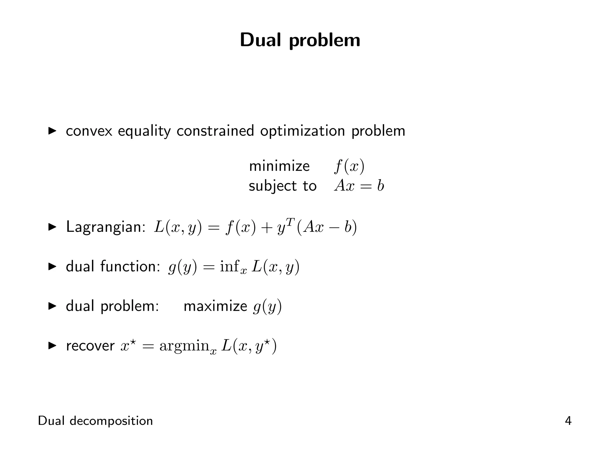
Introduction to convex equality constrained optimization, Lagrangian formulation, and dual problem.
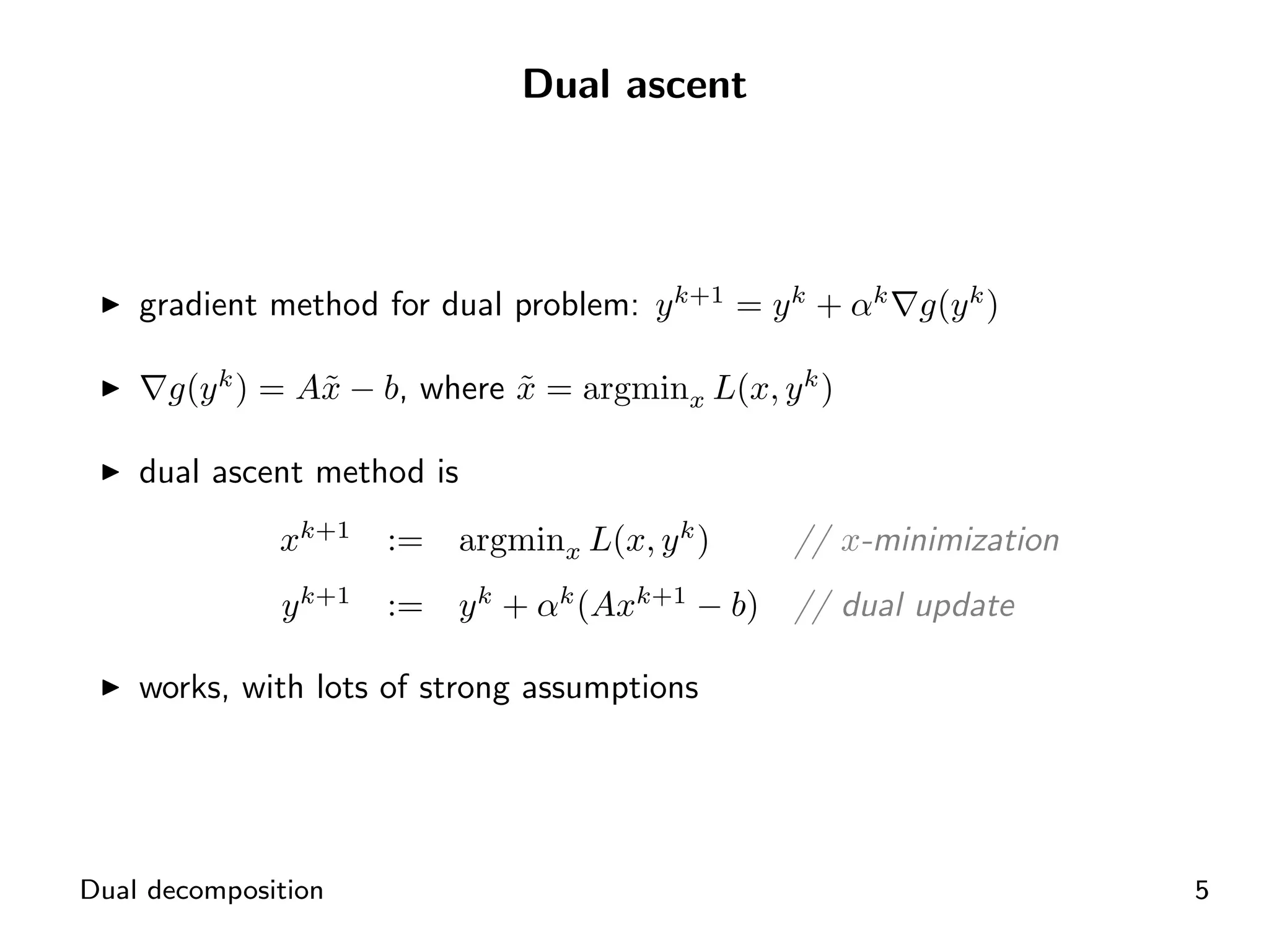
Gradient method for dual problem, outlining dual ascent method updates for variables.
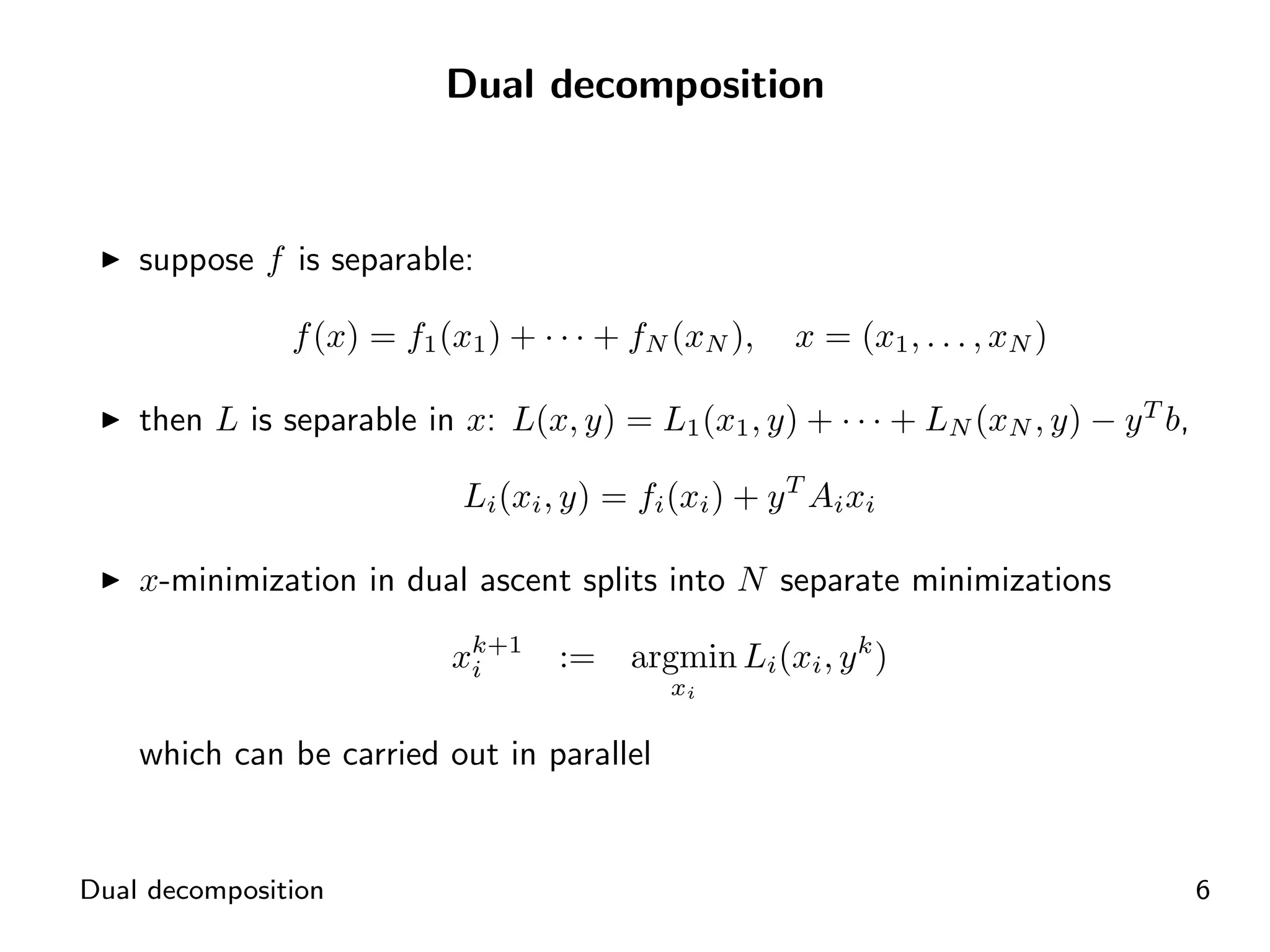
Separate functions allow parallel optimization in dual decomposition.
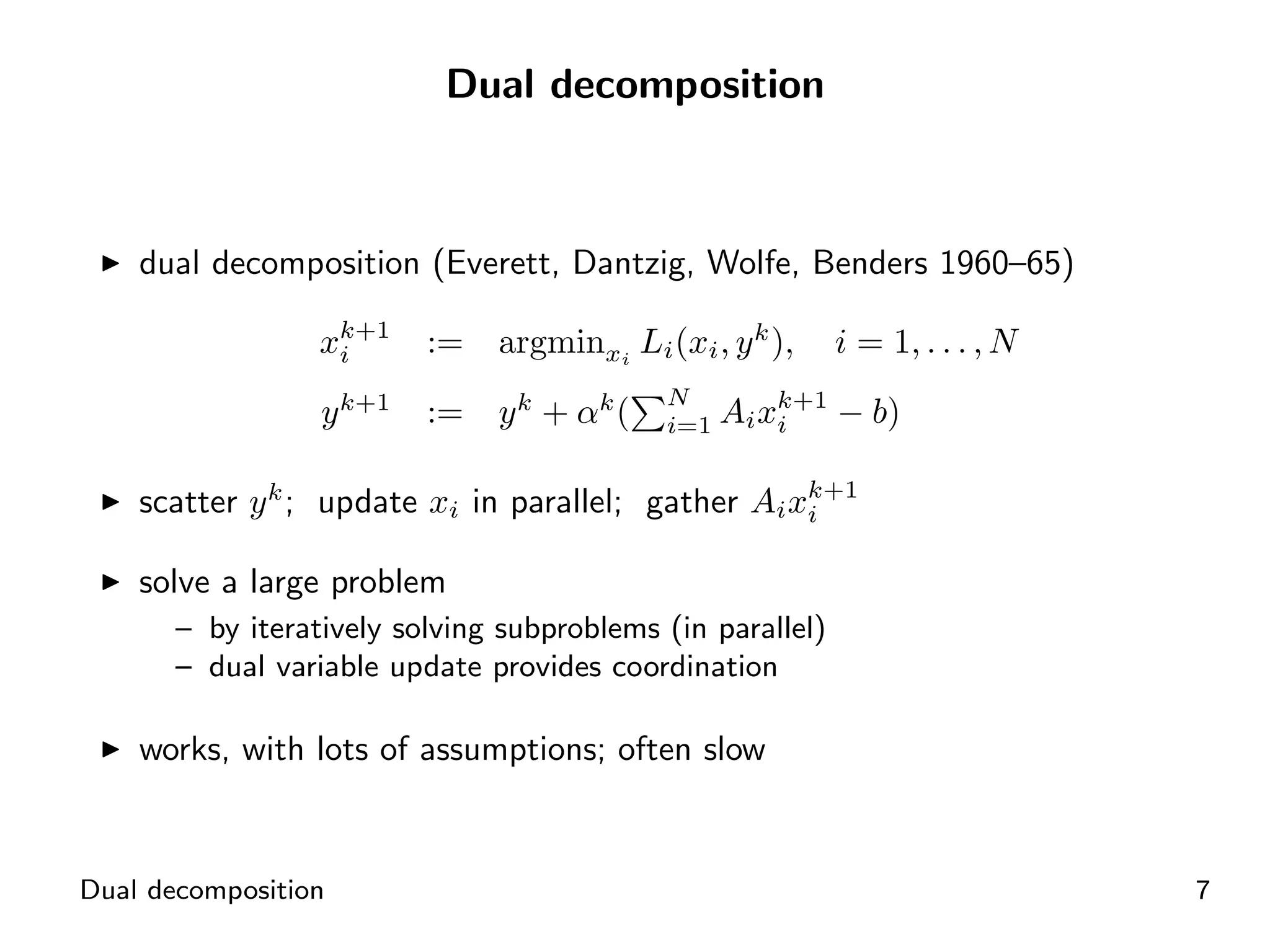
Iterative solving of subproblems in parallel for large problems using dual decomposition.
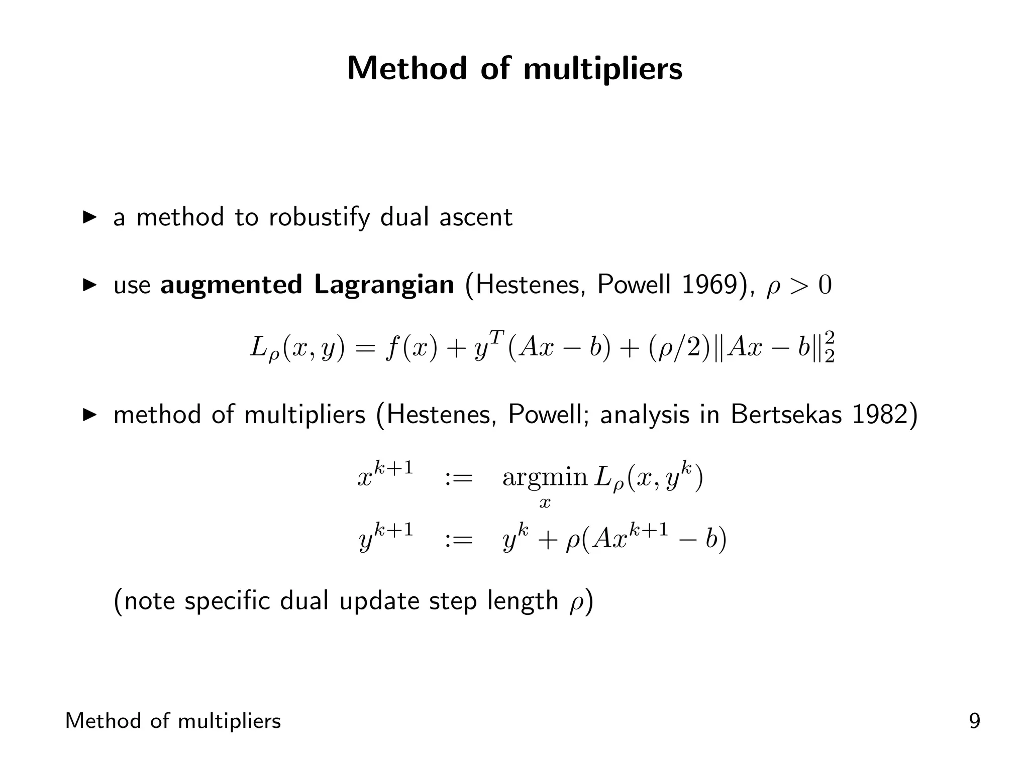
Introduction to the method of multipliers using augmented Lagrangian for dual ascent.
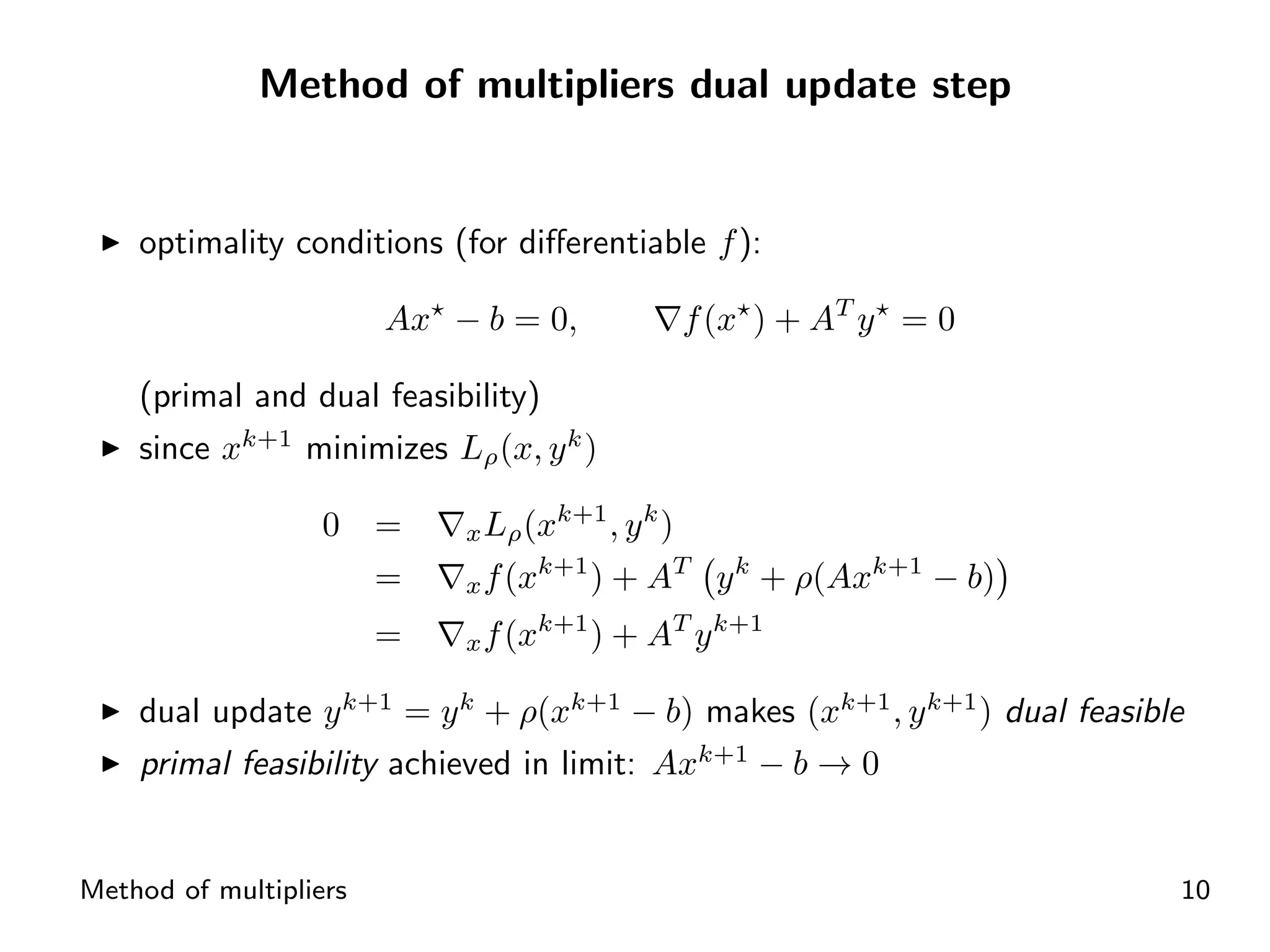
Optimality conditions and dual feasibility through specific update steps in multipliers.
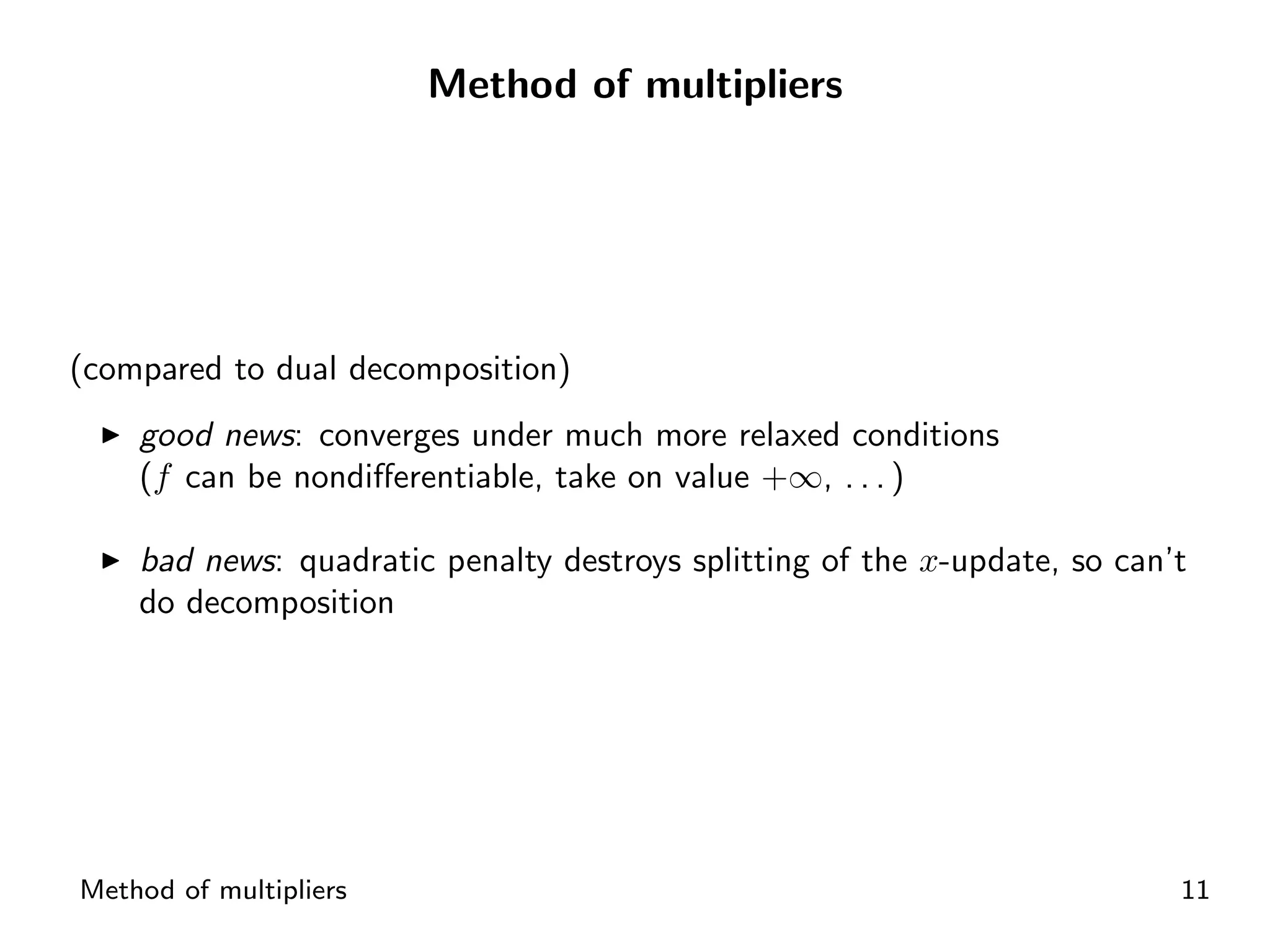
Comparison of dual decomposition and method of multipliers regarding convergence conditions.
Overview of ADMM as a robust method that supports decomposition.
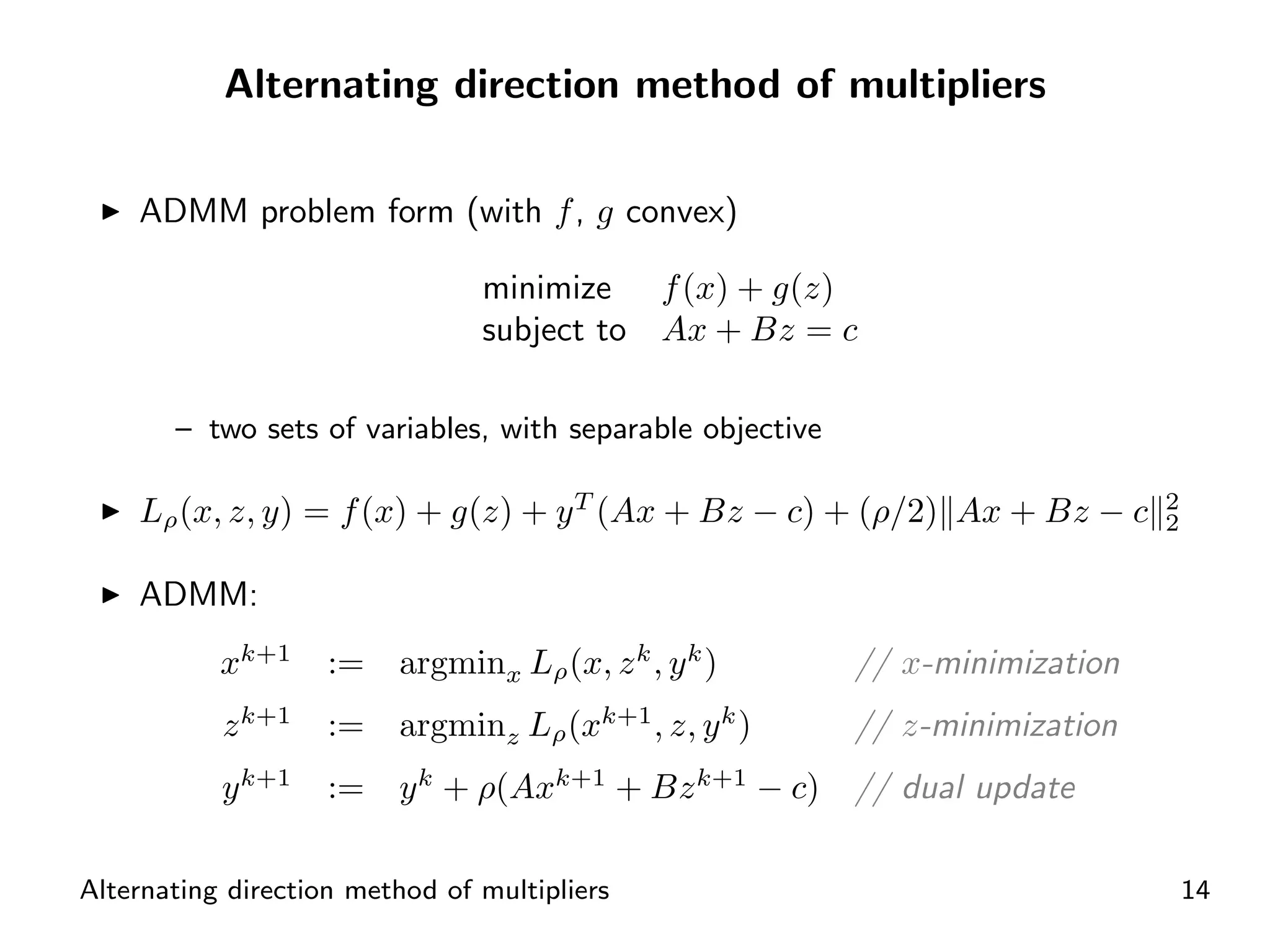
ADMM structure for optimization with convex functions and separable objectives.
Underlines the one pass of Gauss-Seidel in minimizing over variables in ADMM.
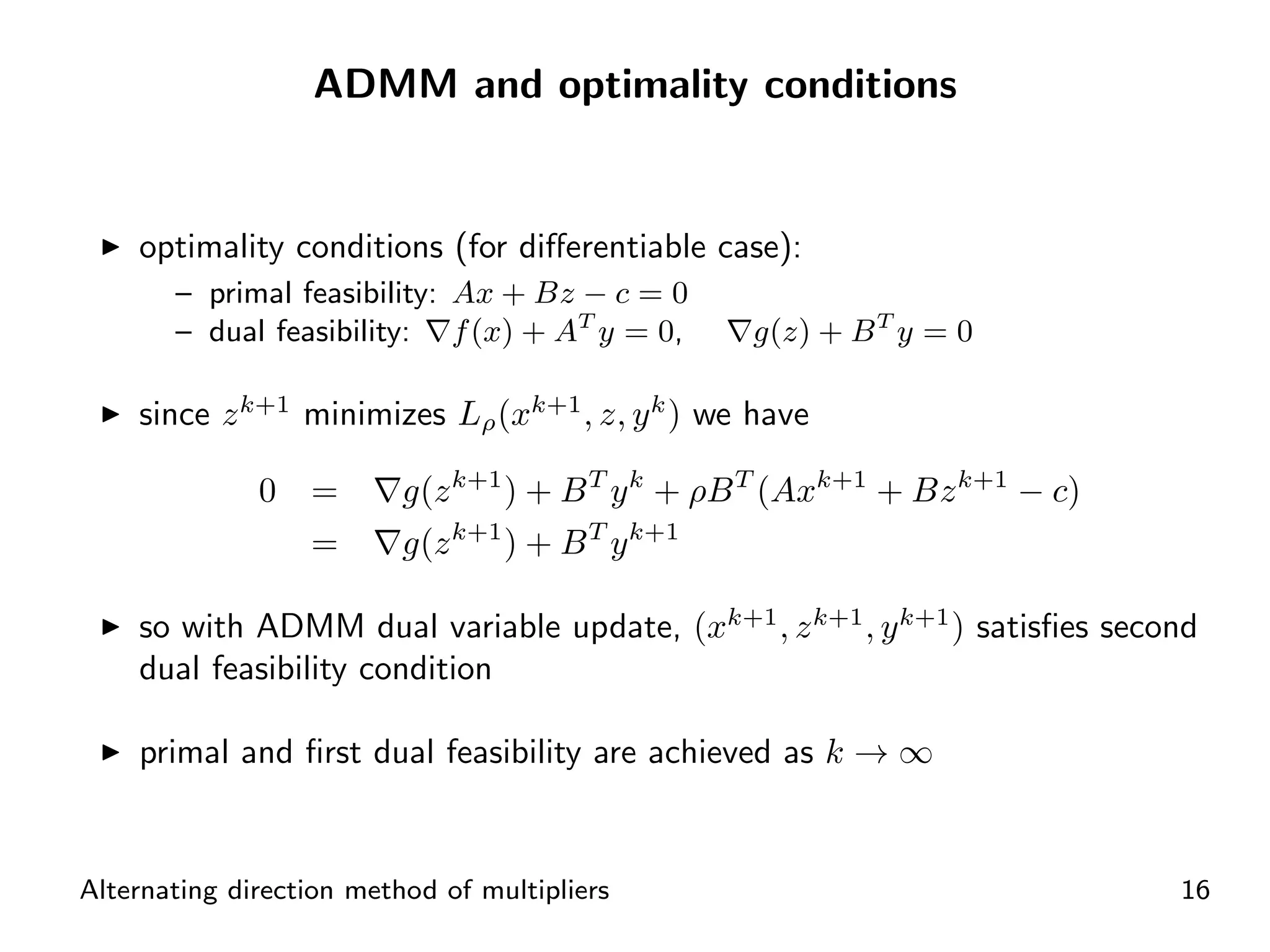
Optimality conditions for convergence in ADMM regarding both primal and dual feasibility.
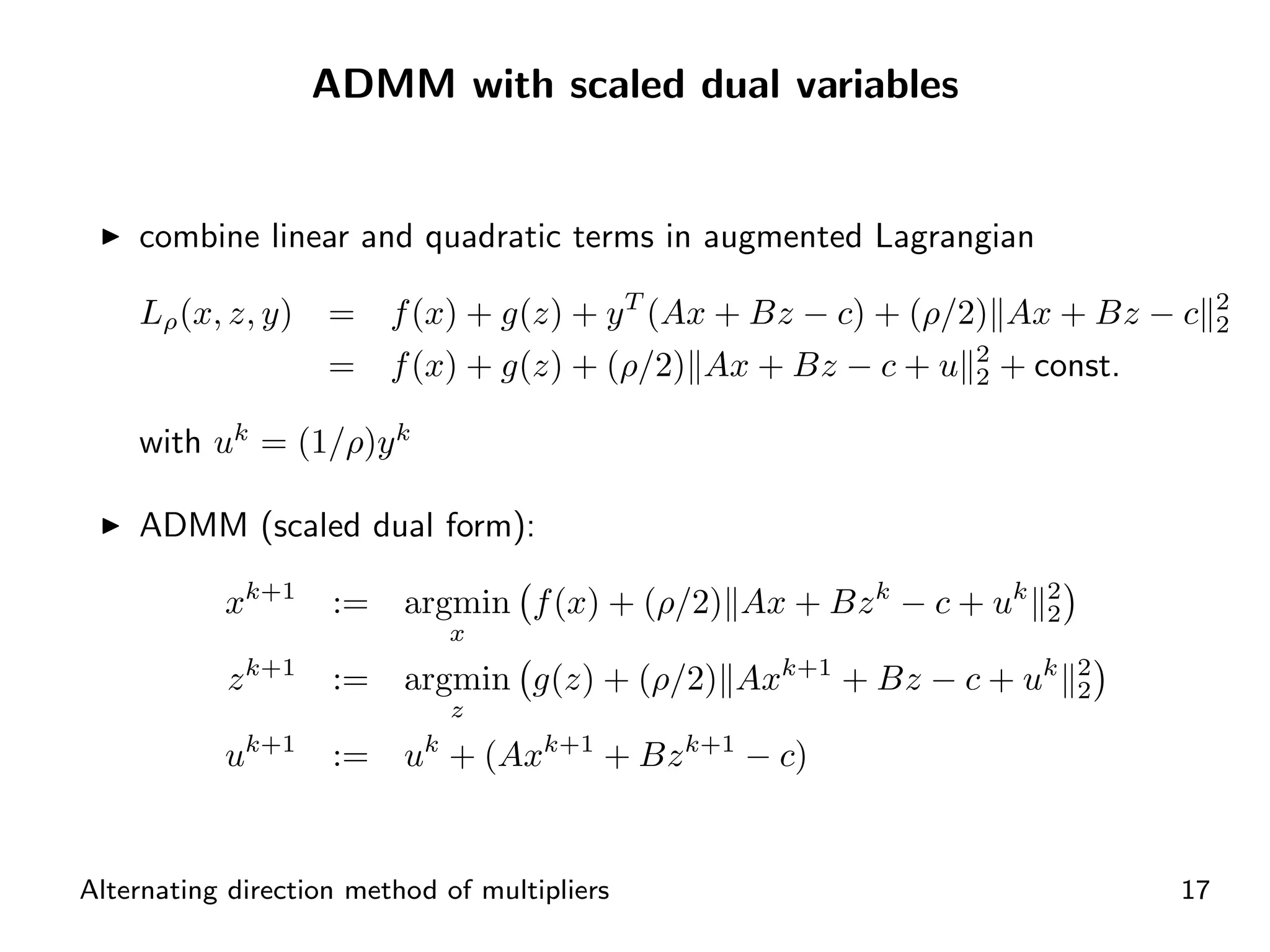
Inclusion of scaled dual variables in ADMM for improved convergence and performance.
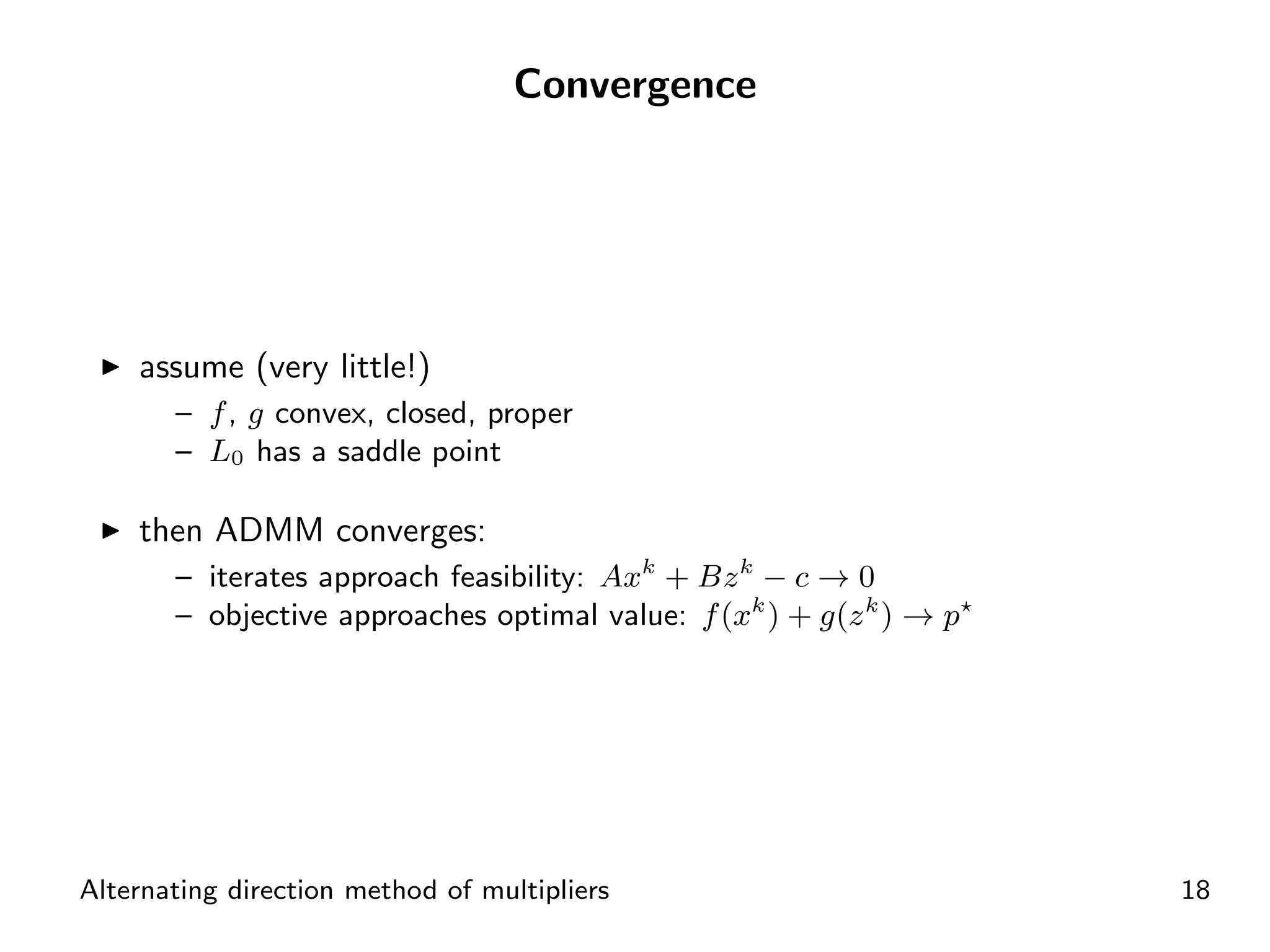
Convergence assumptions for ADMM ensuring optimal value approach and feasibility.
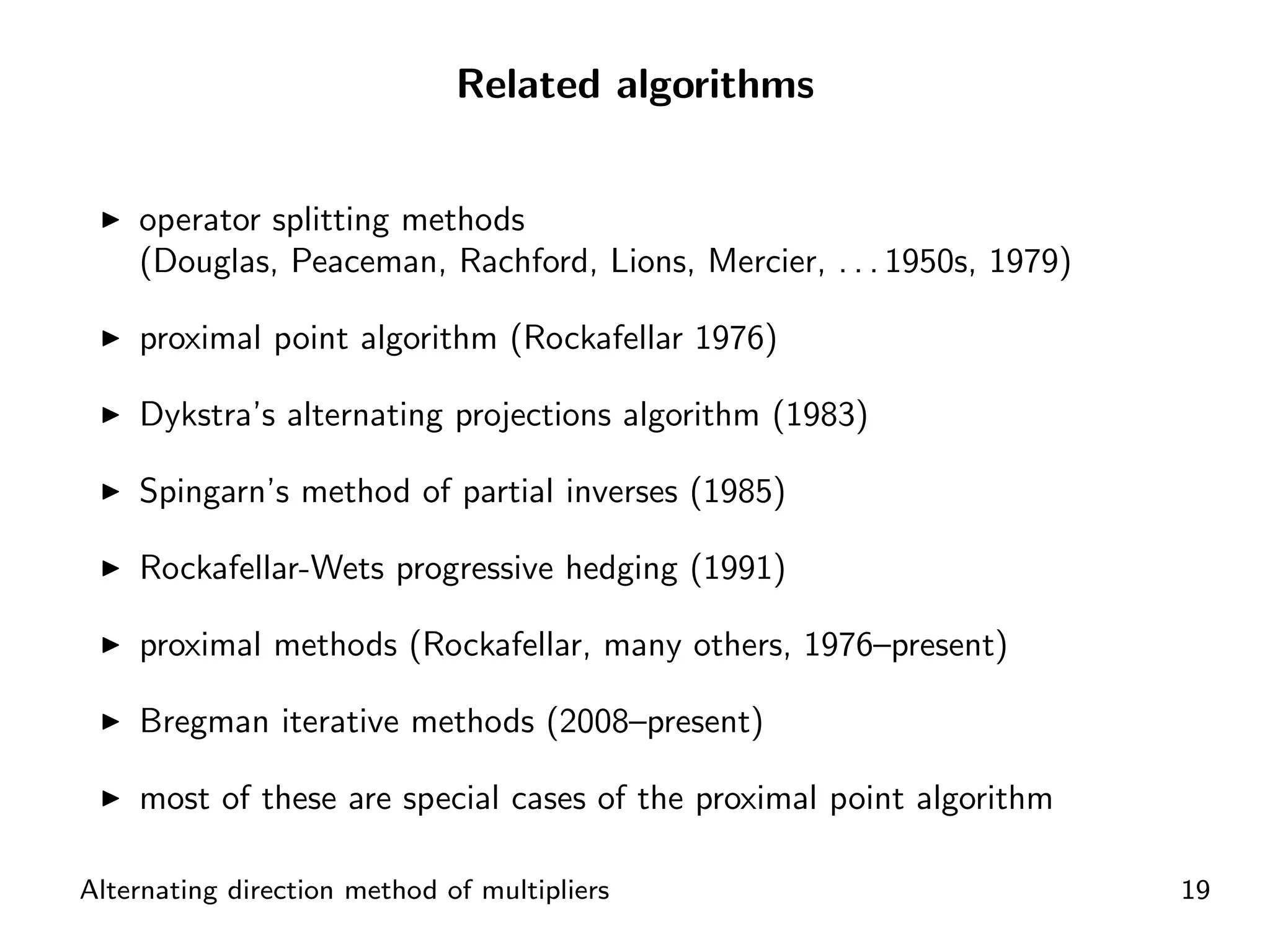
Connections to operator splitting methods, proximal point algorithm, and variations.
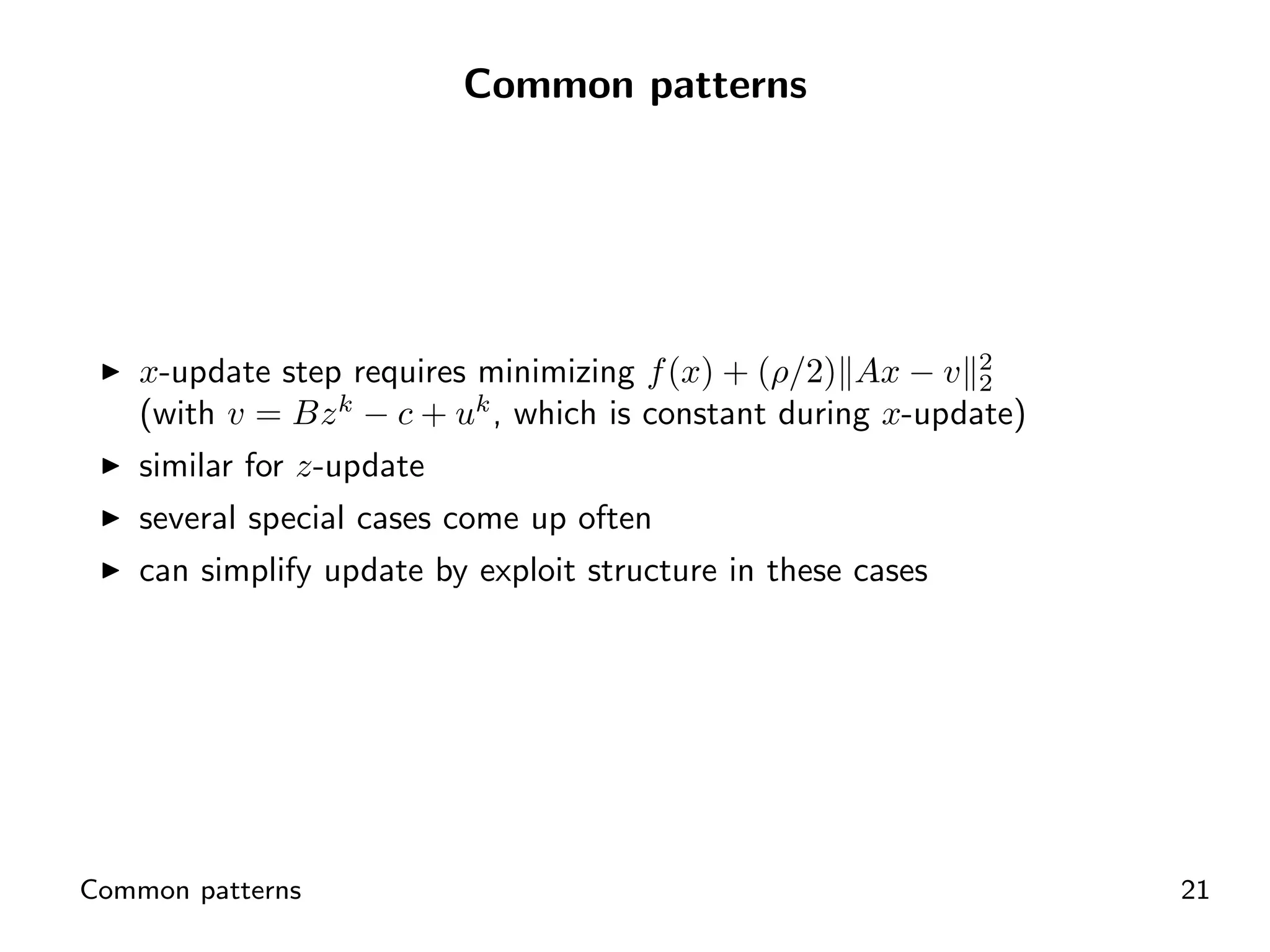
Review of common patterns observed in updates during optimization processes.
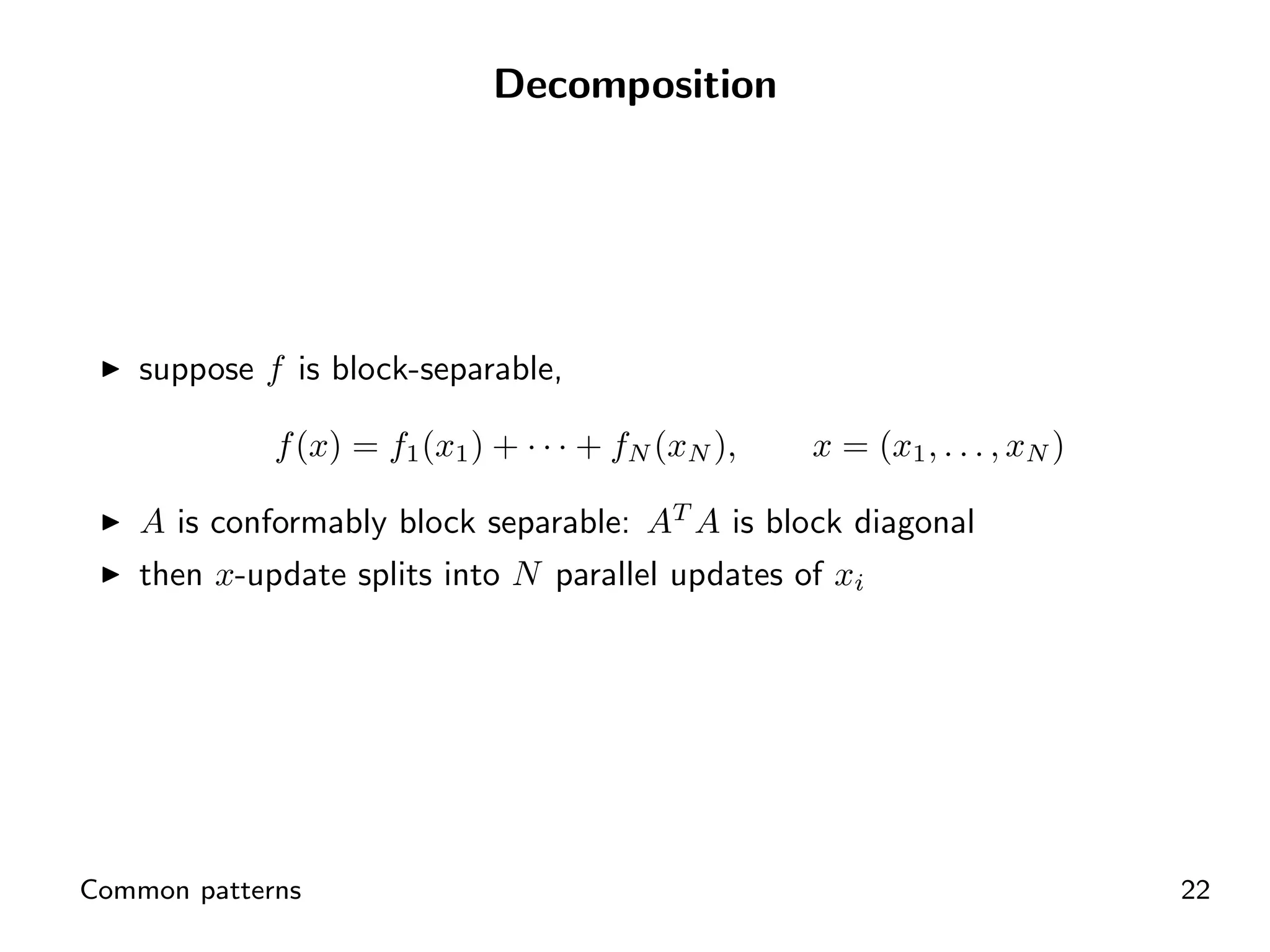
Insights into block-separability in optimization and implications for parallel operations.
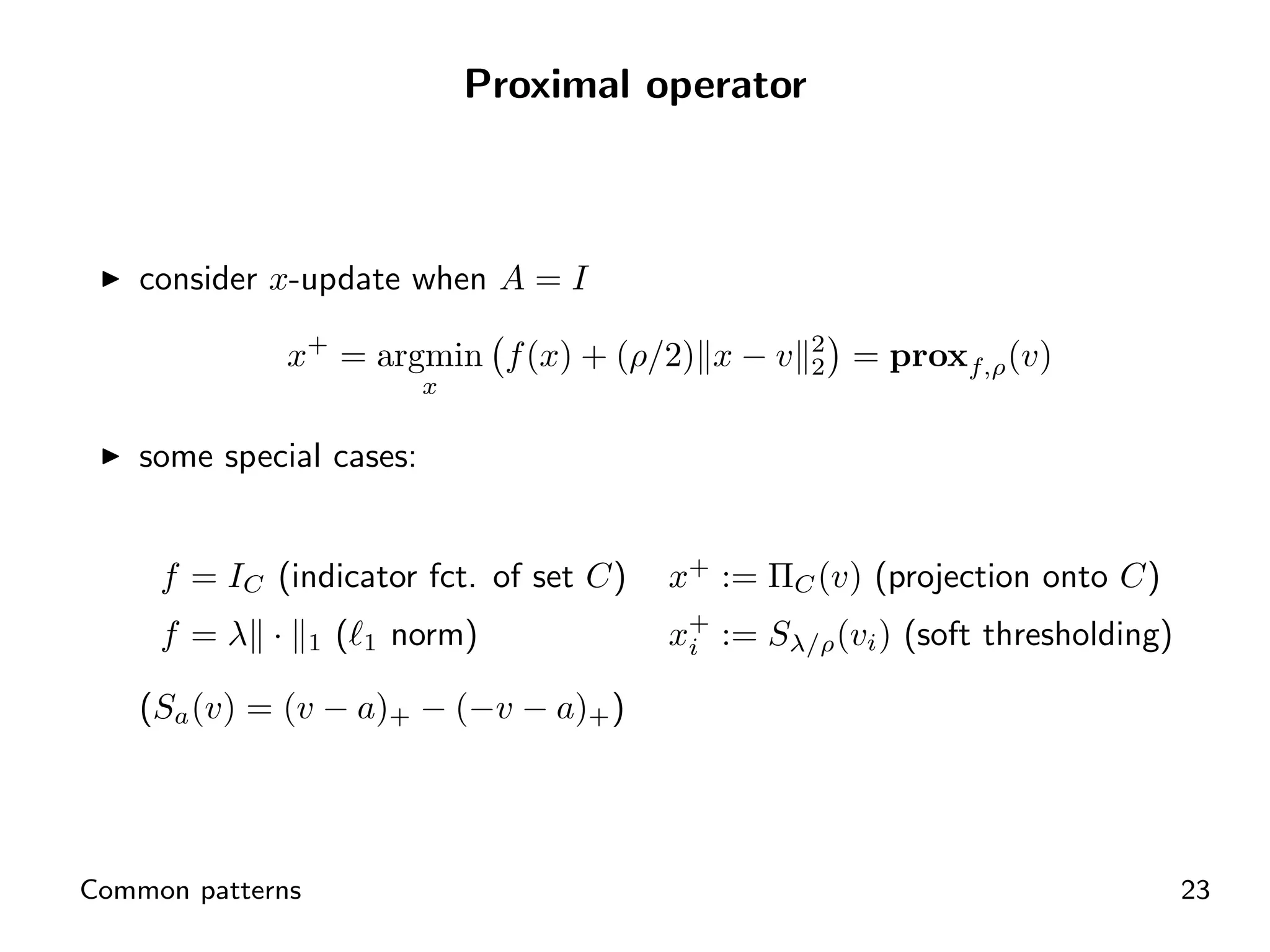
Application of proximal operators in specific optimization updates.
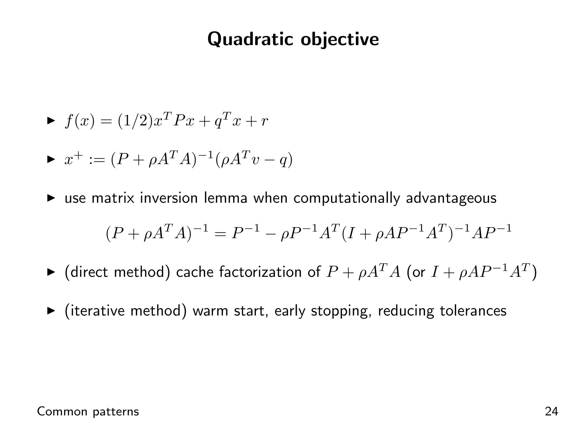
Method for handling updates in quadratic objectives using matrix inversion.
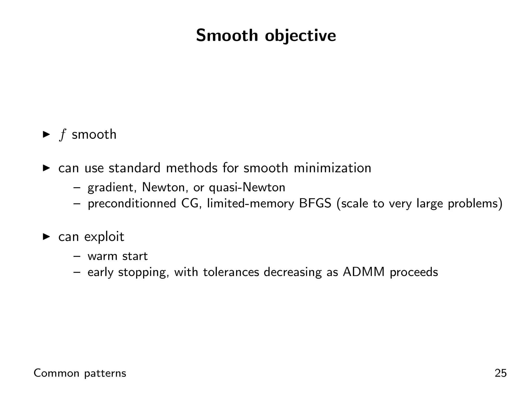
Utilizing efficient methods like gradient or Newton for smooth objective functions.
Practical examples showcasing the implementation of ADMM in optimization scenarios.
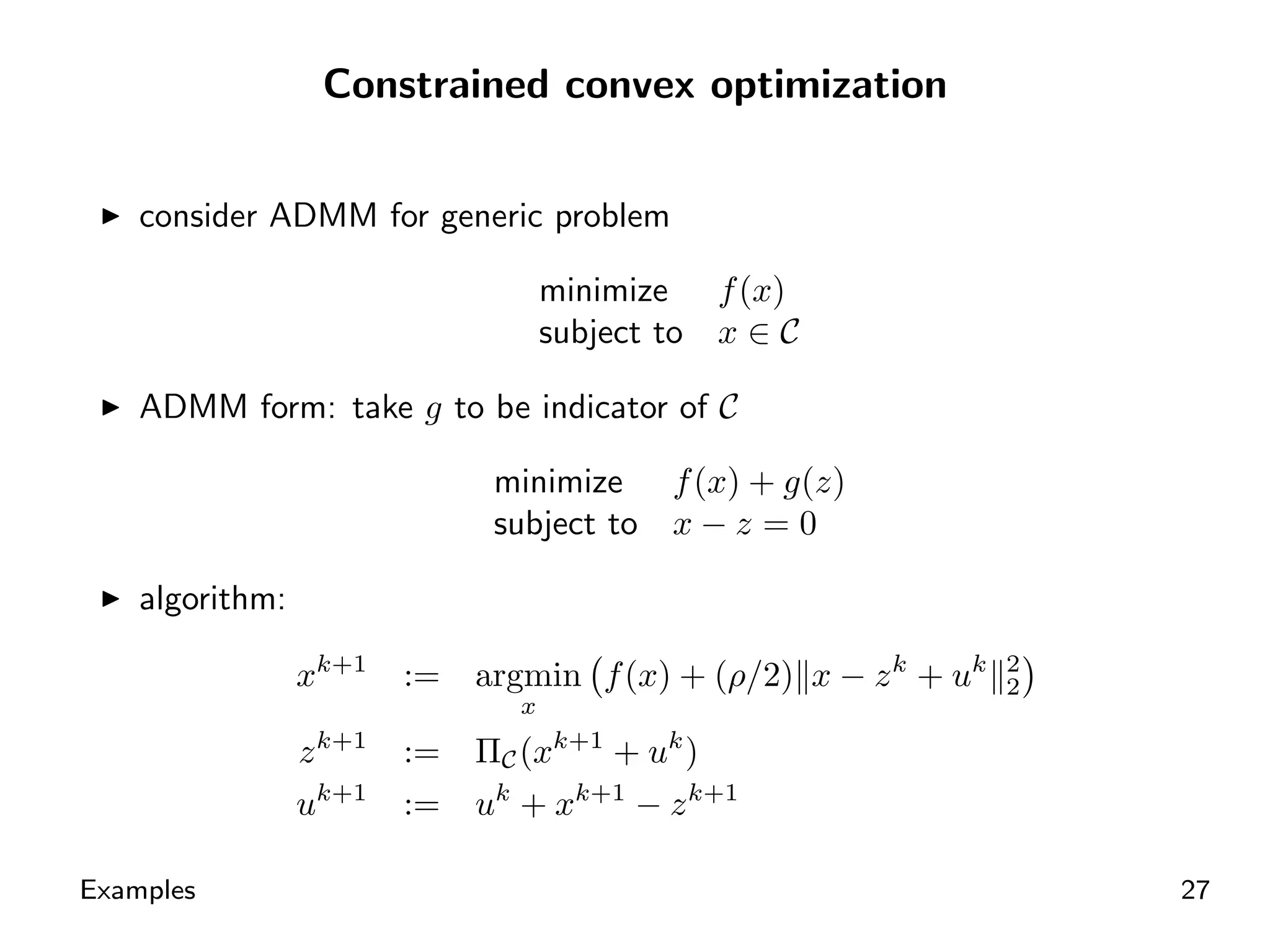
ADMM application in constrained convex optimization with indicator functions.
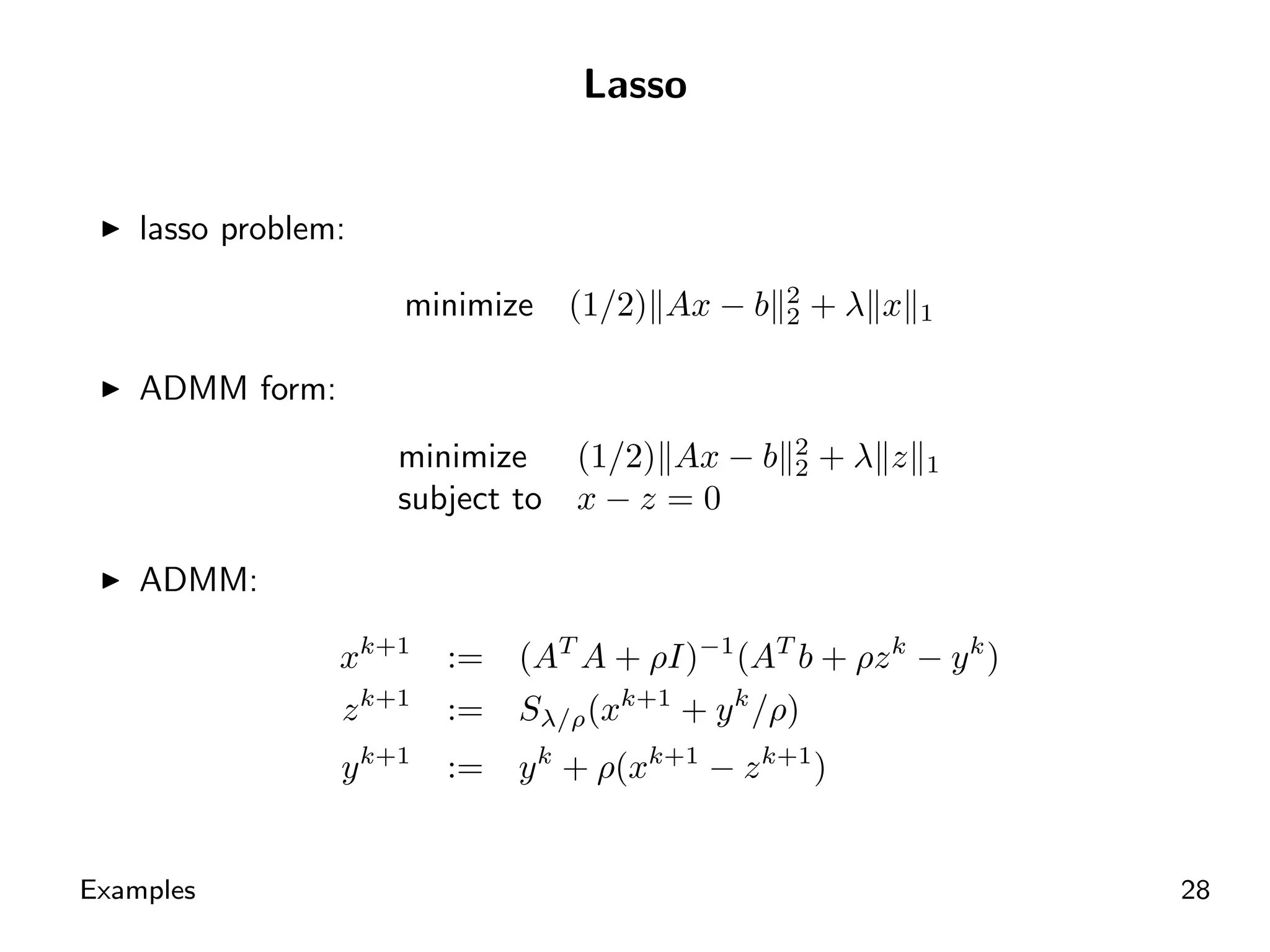
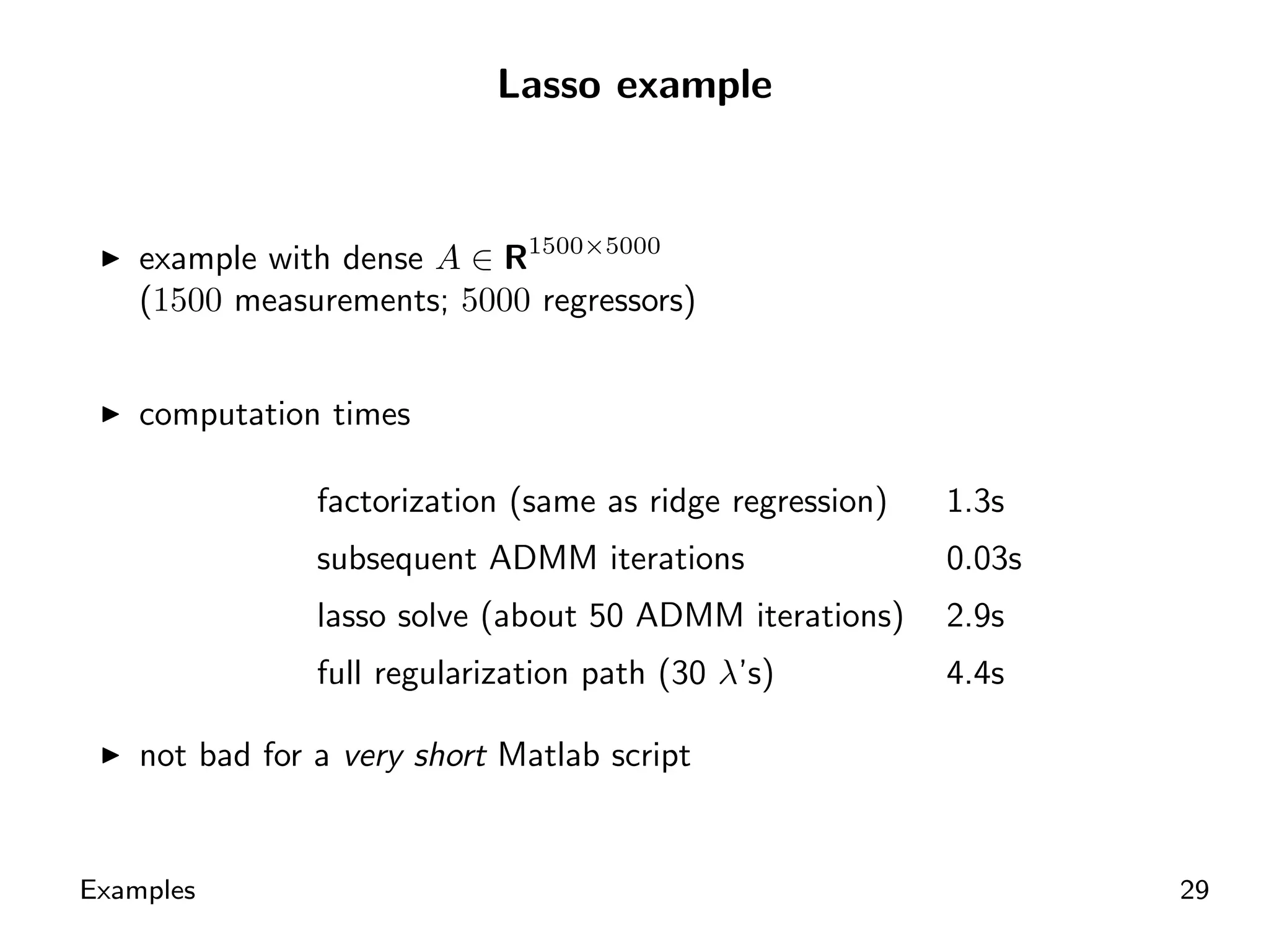
Structured Lasso optimization problem leveraging ADMM for solution.
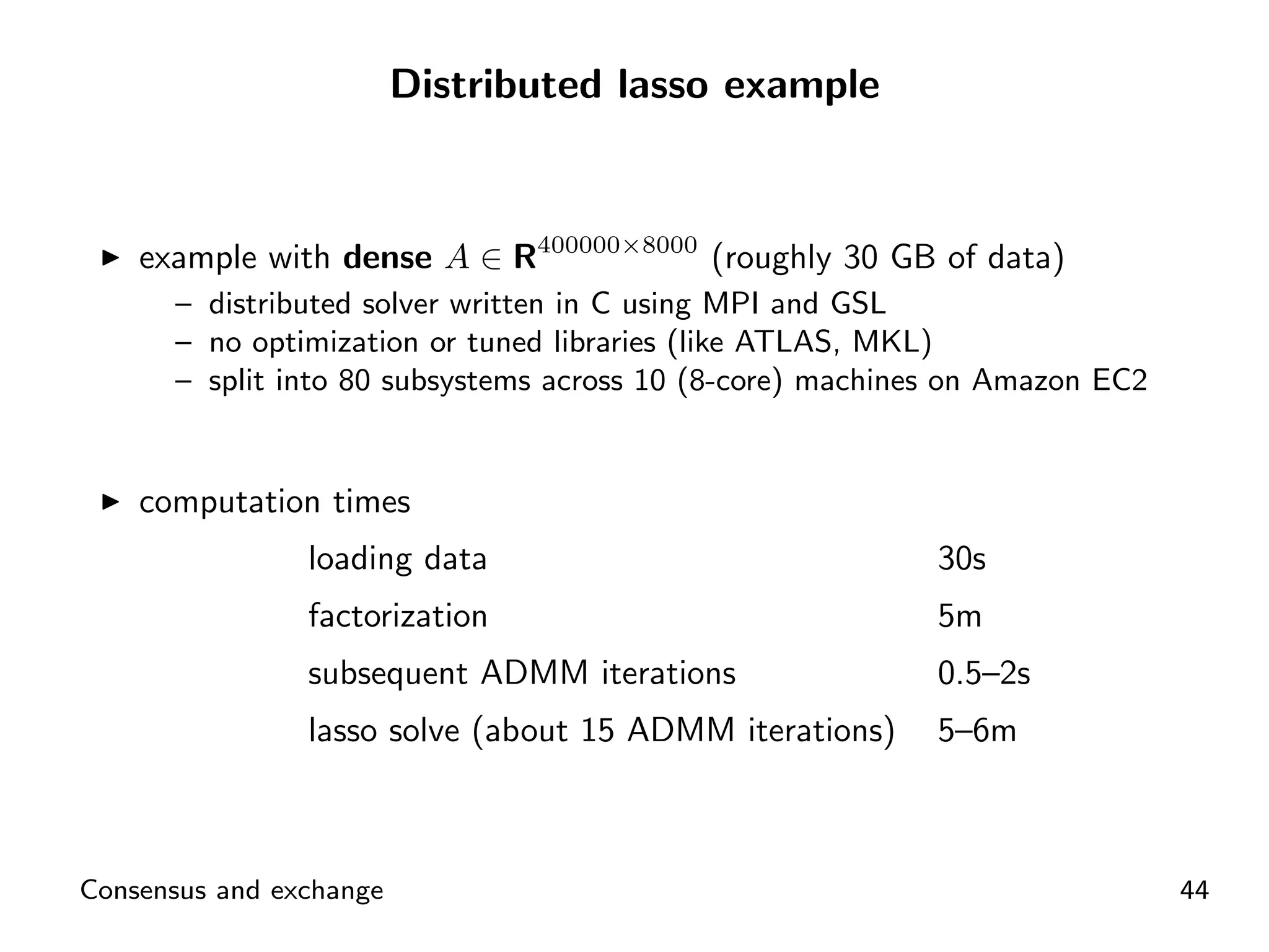
Computational efficiency for Lasso problem exhibited through various runtime metrics.
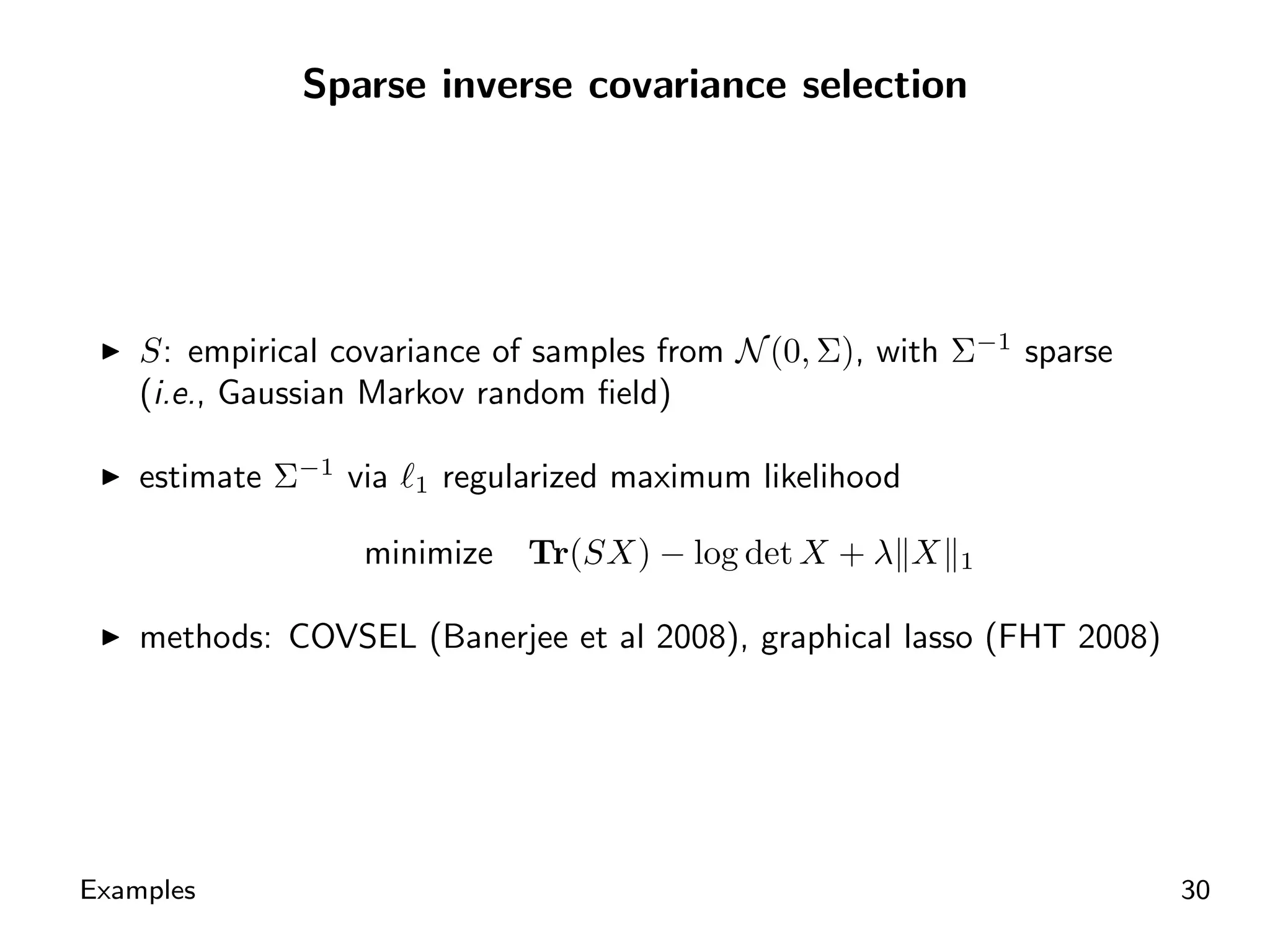
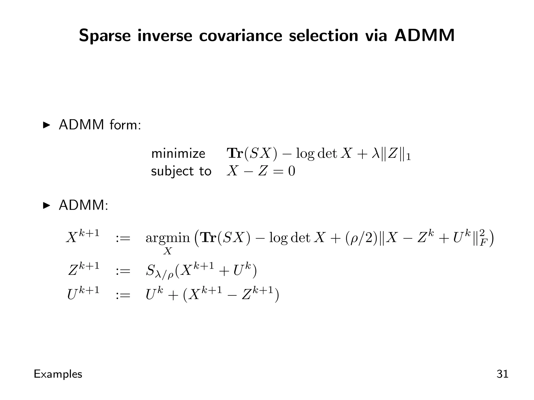
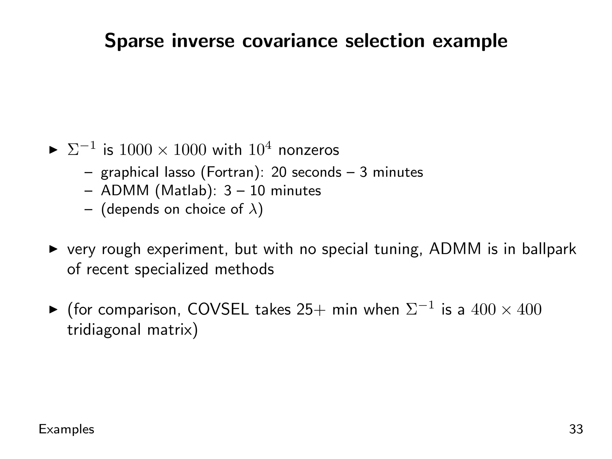
ADMM framework employed for estimating sparse inverse covariance in statistical models.
Algorithmic steps for sparse inverse covariance selection with ADMM.
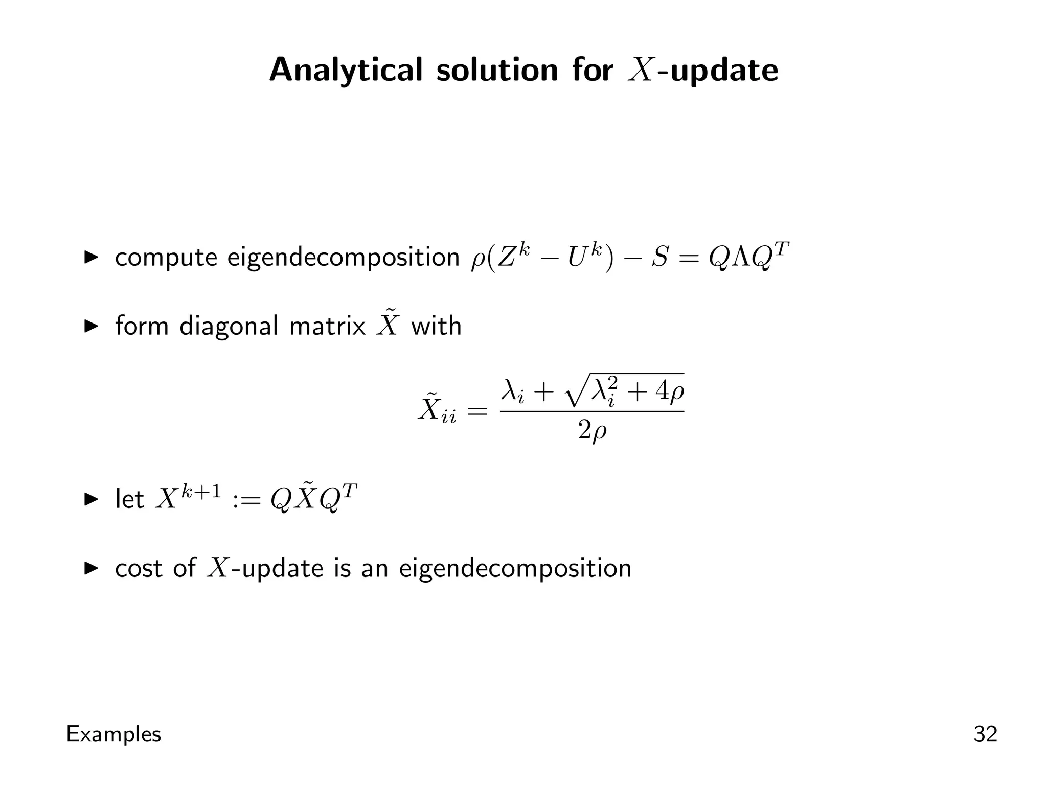
Employing eigendecomposition in ADMM for efficient X-update computations.
Efforts to benchmark ADMM's performance against specialized methods for sparse covariance.
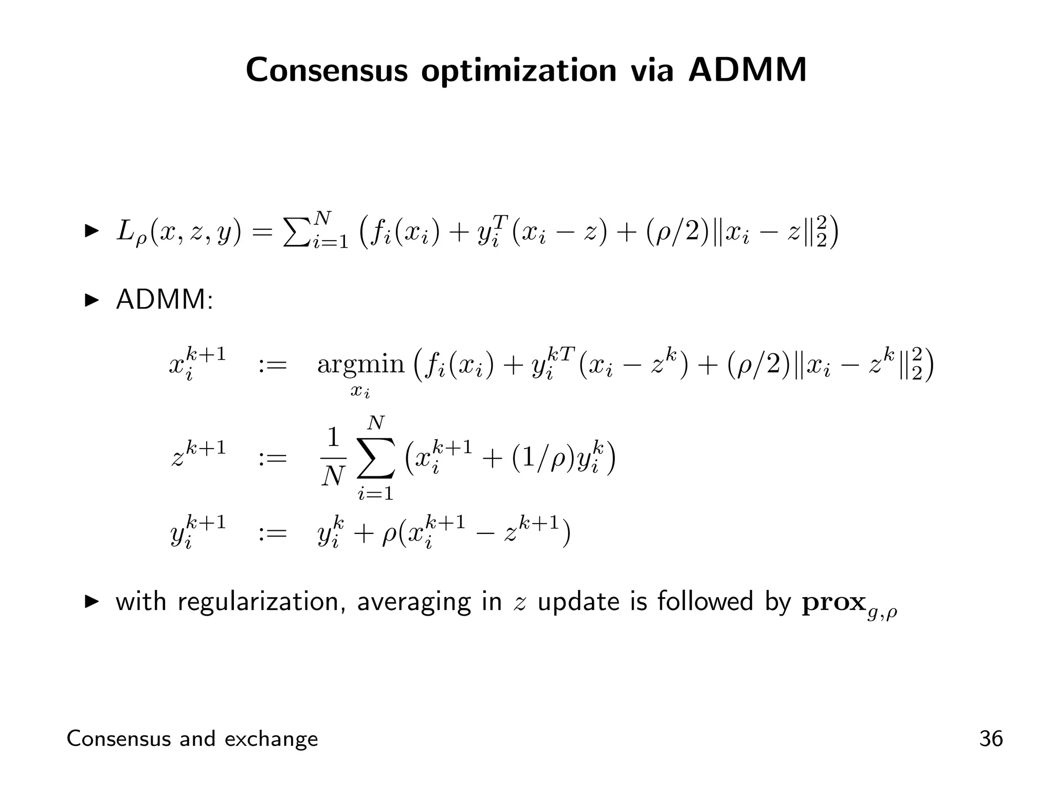
Introduction to consensus optimization focusing on minimizing multiple objective terms.
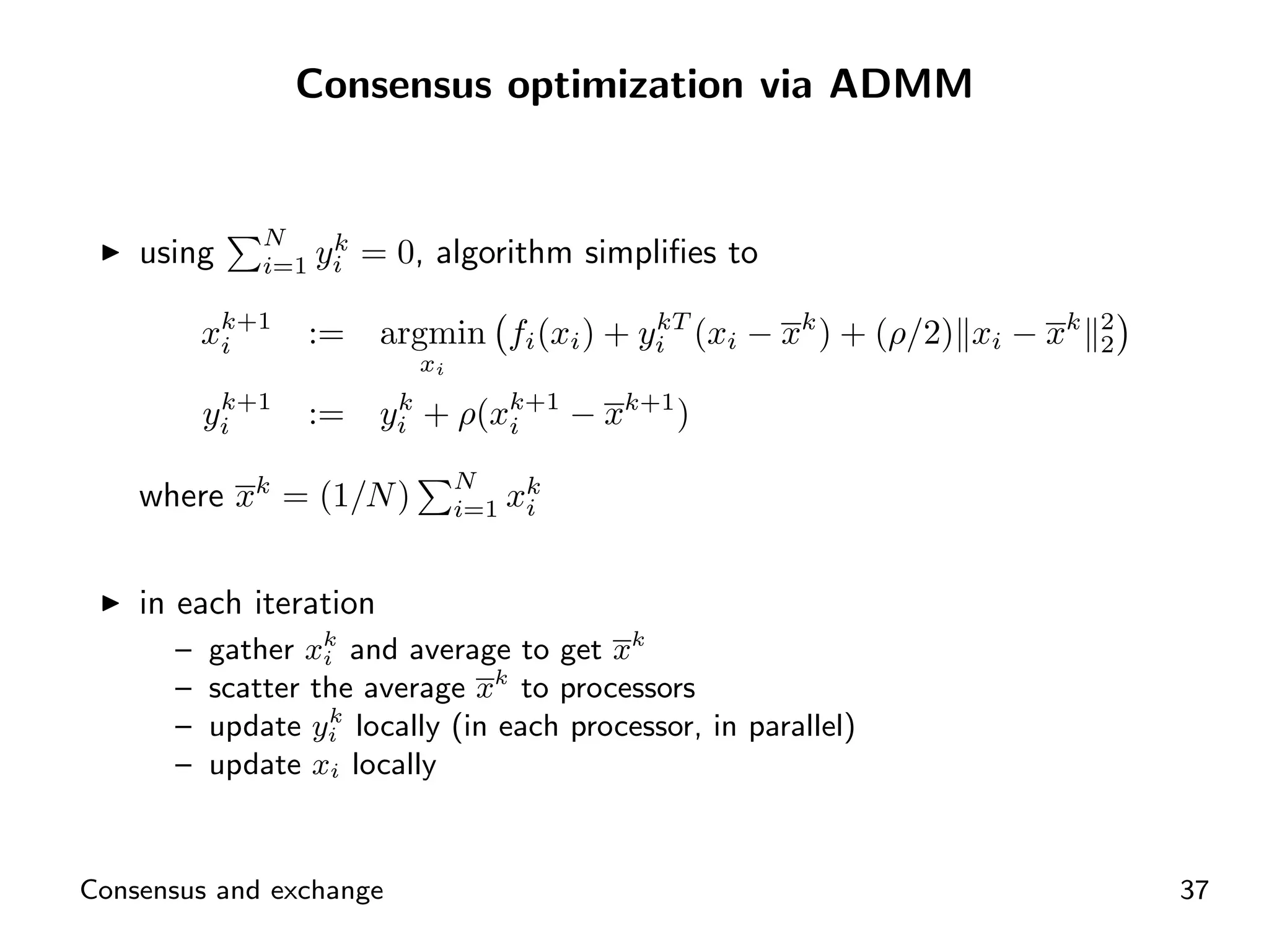
Implementation of ADMM for solving consensus optimization through local and global variables.
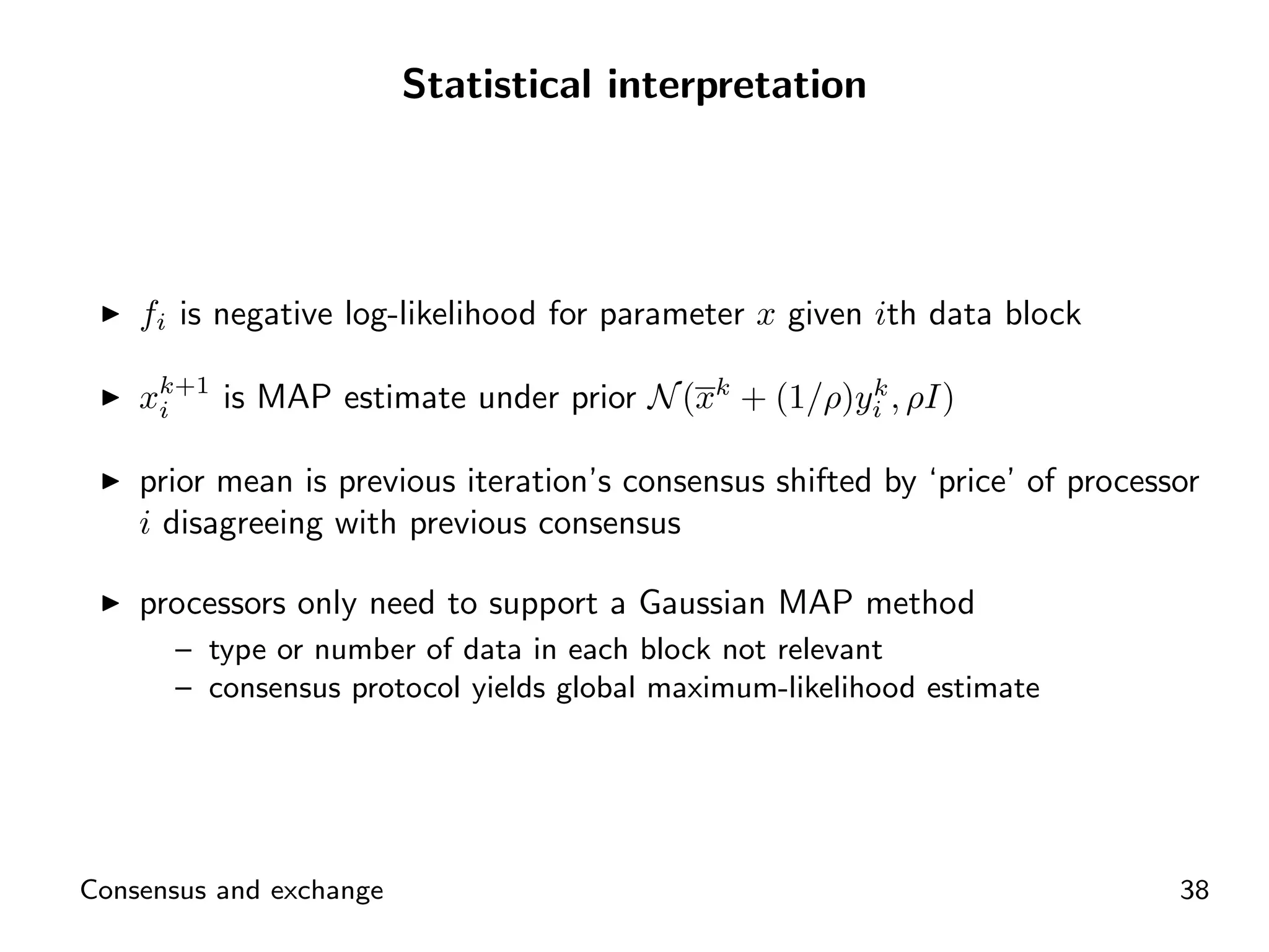
Interpreting consensus in statistical terms related to maximum likelihood estimation.
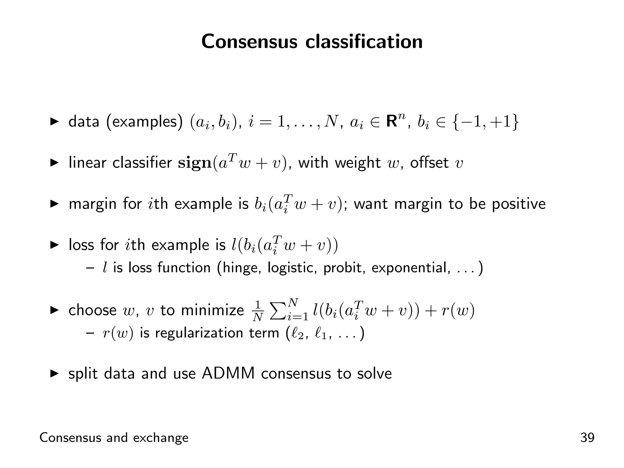
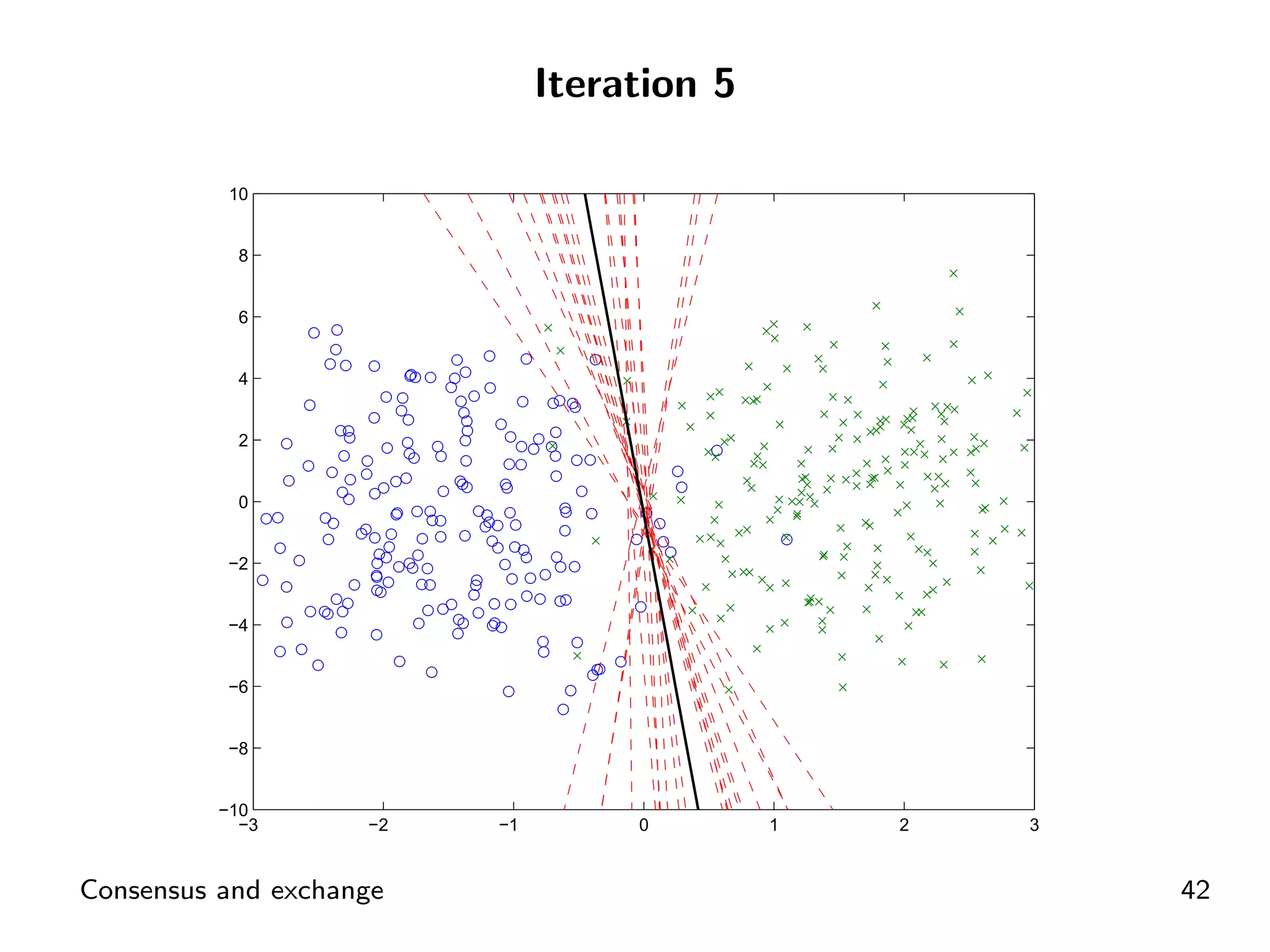
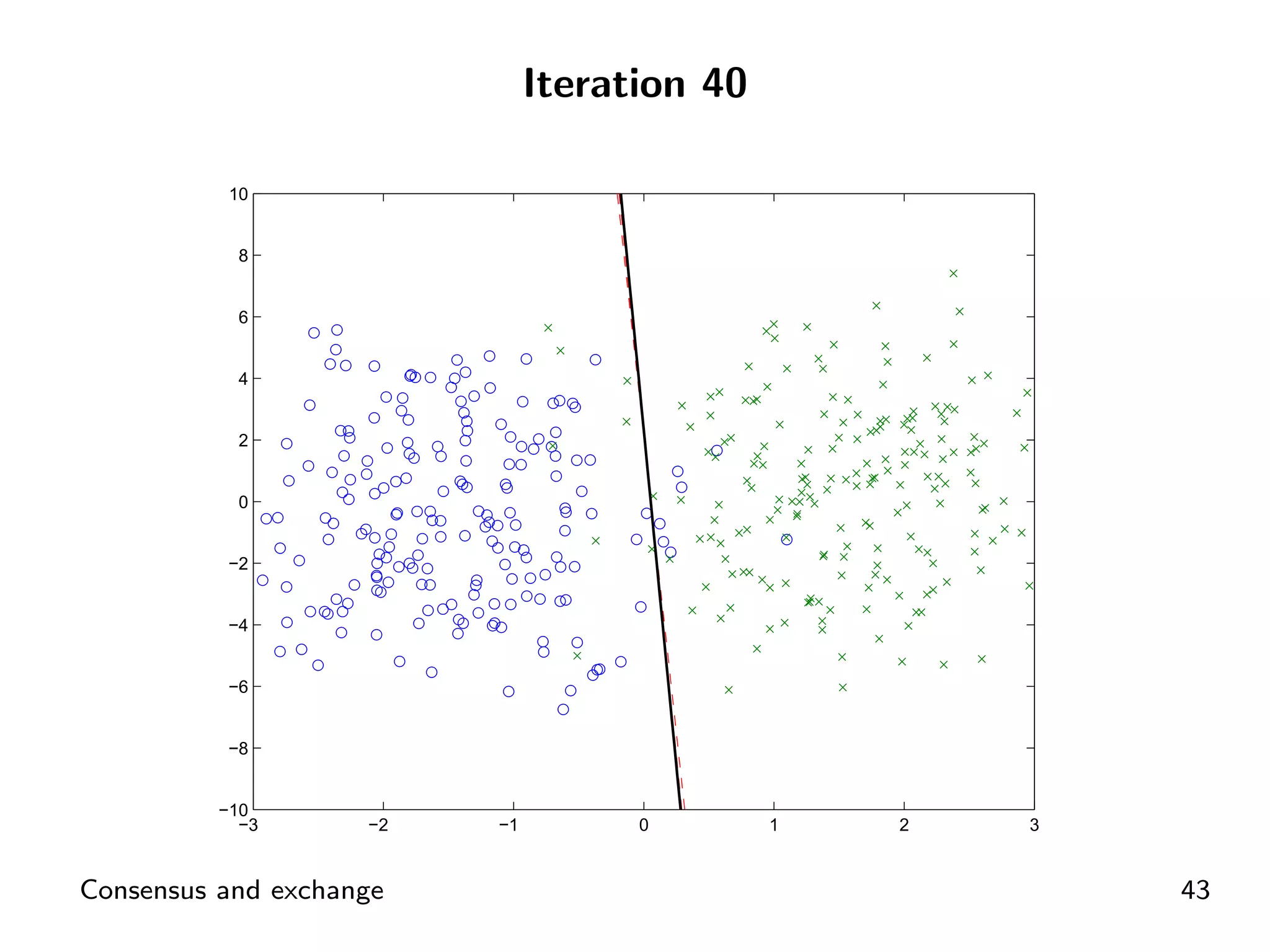
Defining consensus classification problems using loss functions for optimization.
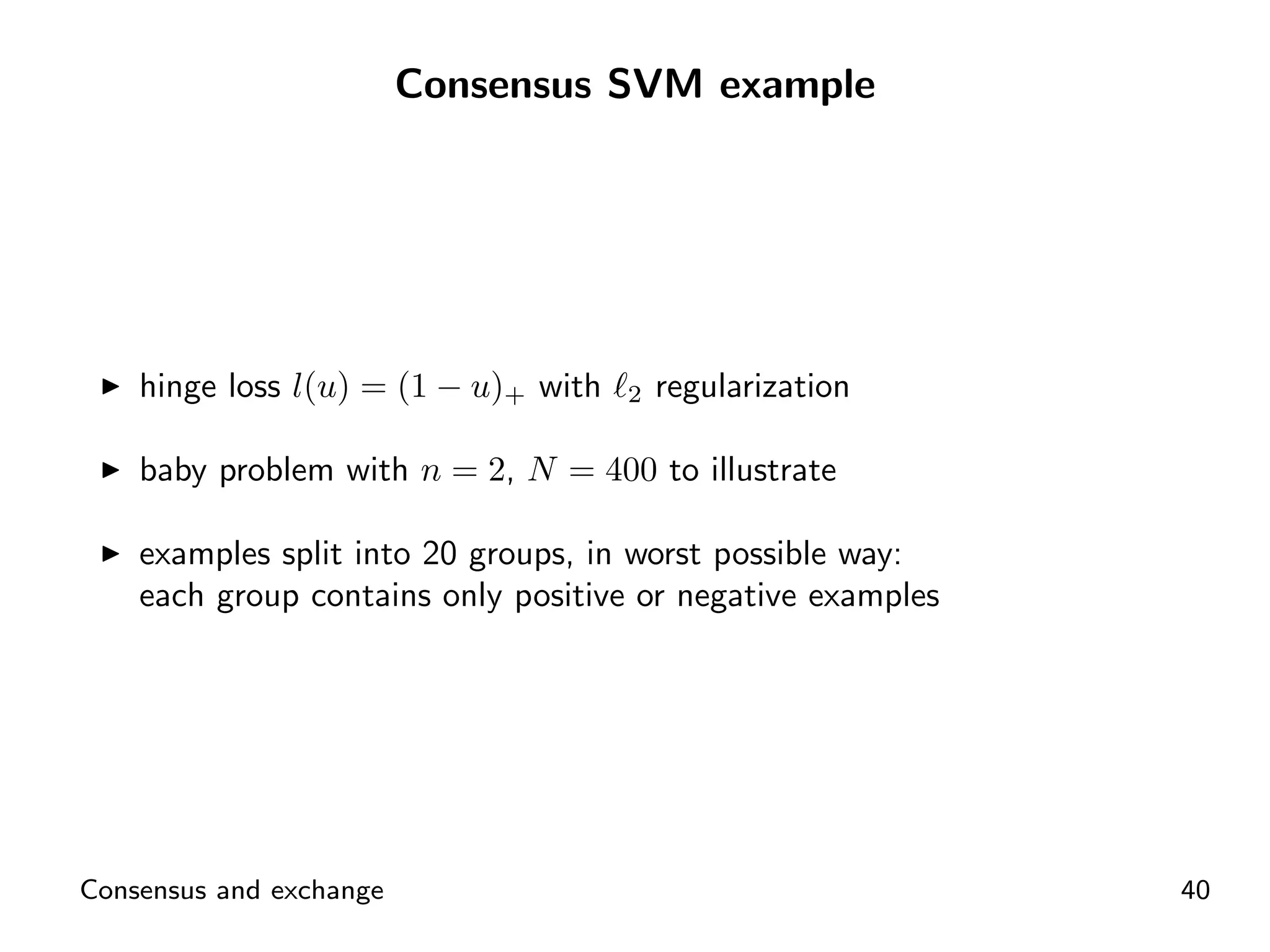
Example layout demonstrating consensus in SVM problems through ADMM.
Handling large datasets through distributed approaches in Lasso problems using ADMM.
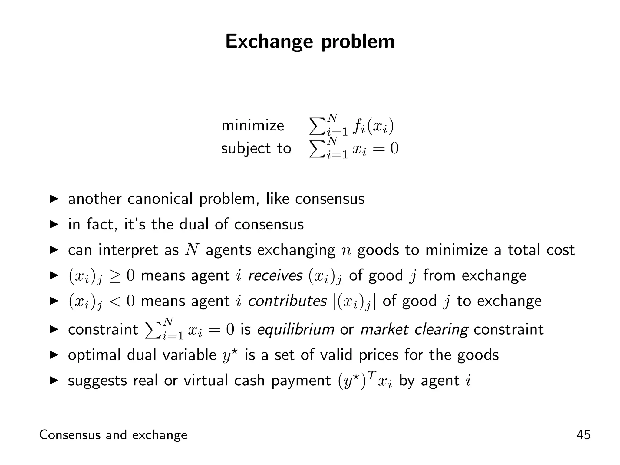
Introductory concepts and expressions related to agents exchanging goods and costs.
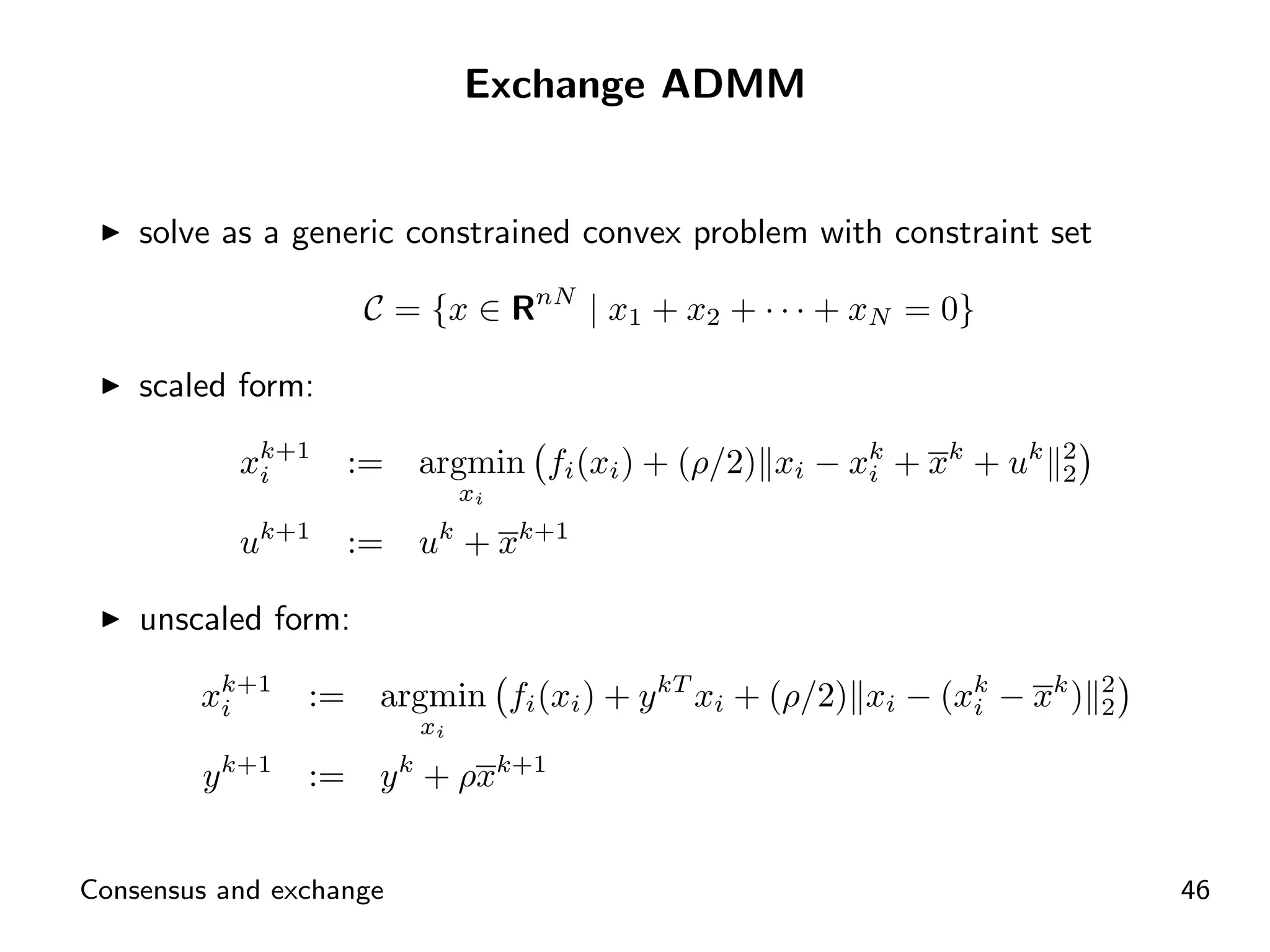
Utilizing ADMM framework to solve exchange problems with unique constraints.
Examining the exchange problem through the lens of market equilibrium processes.
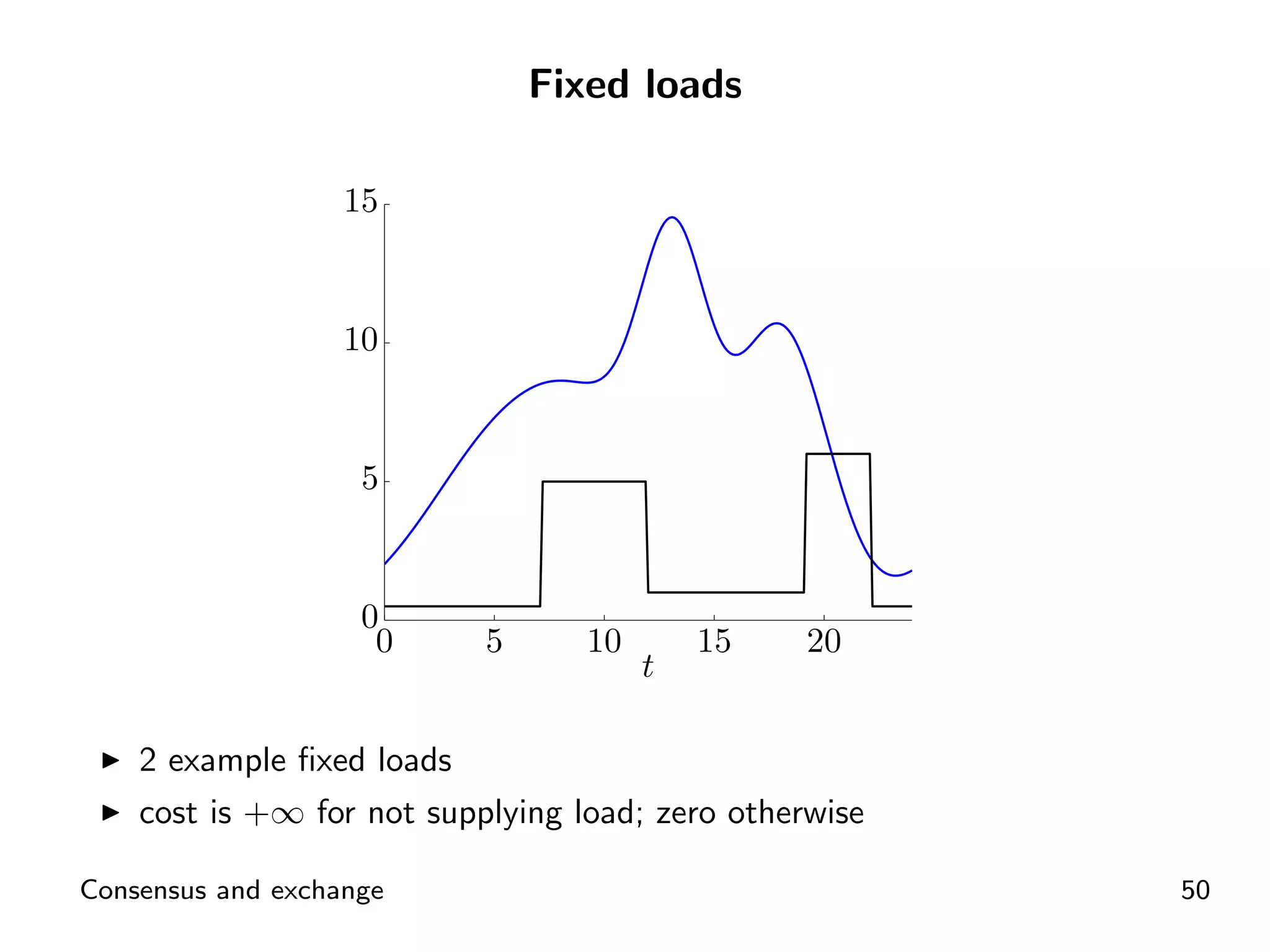
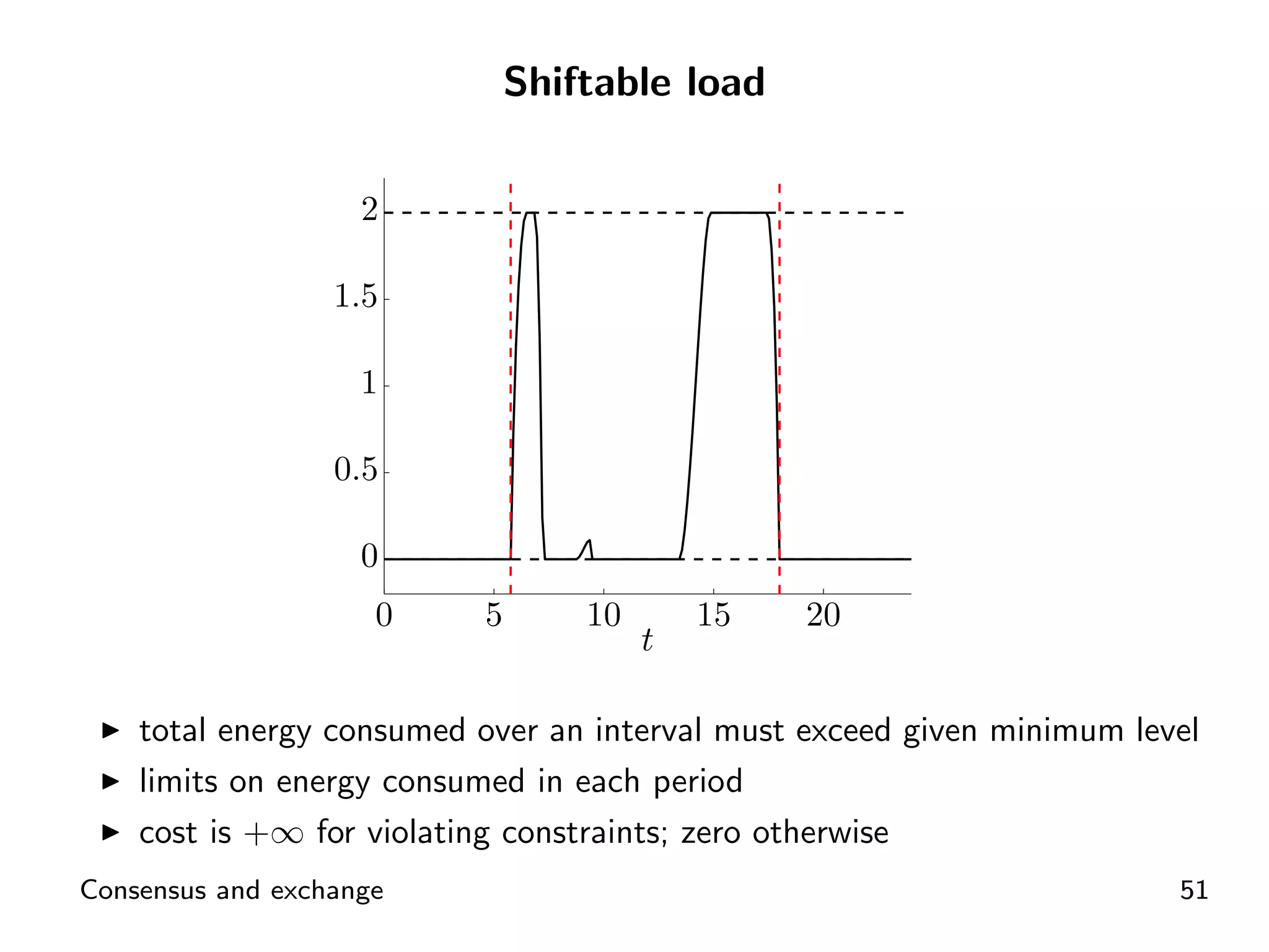
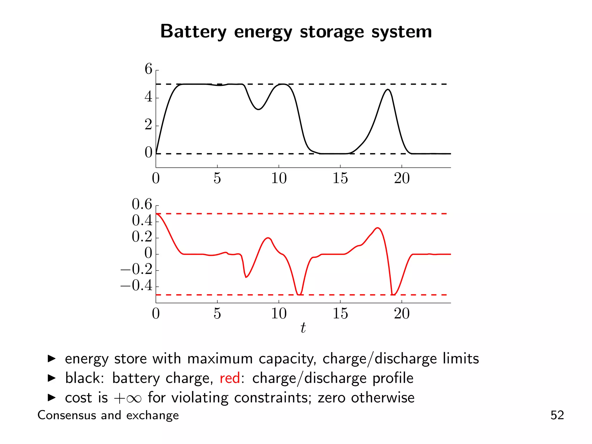
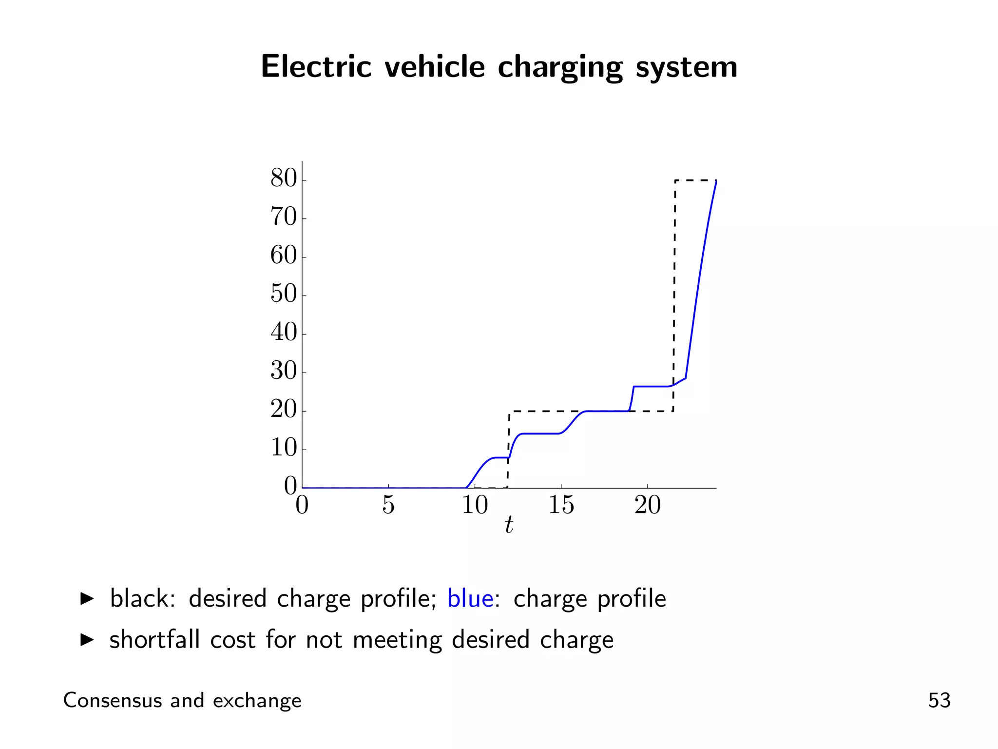
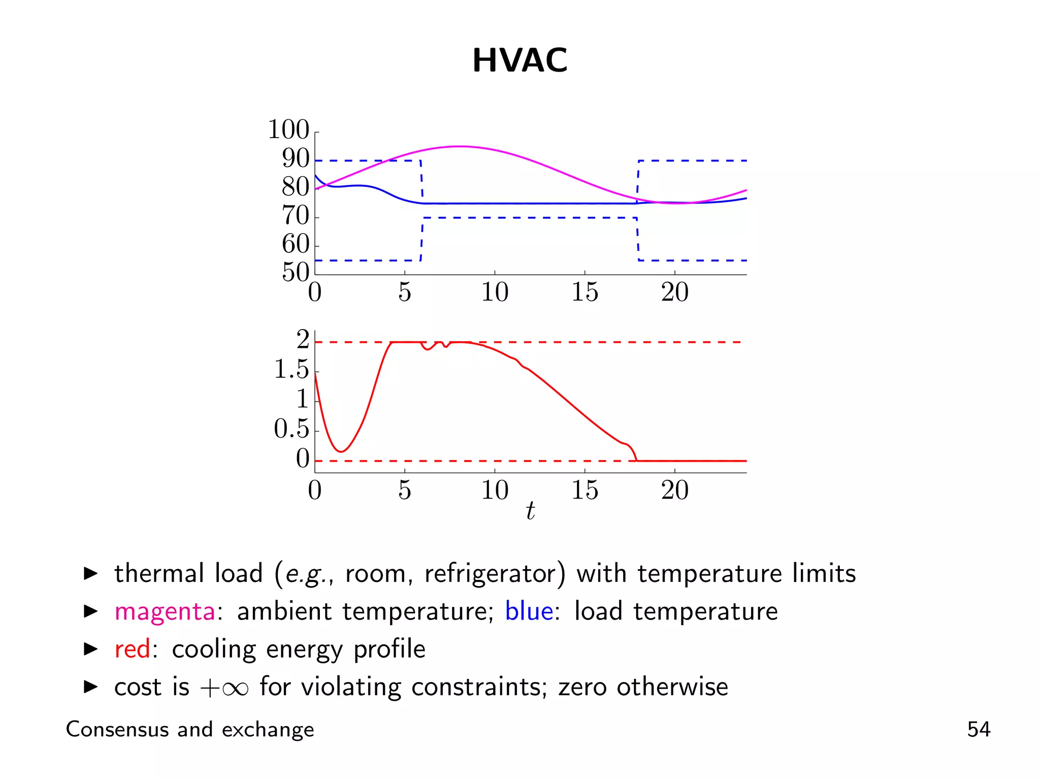
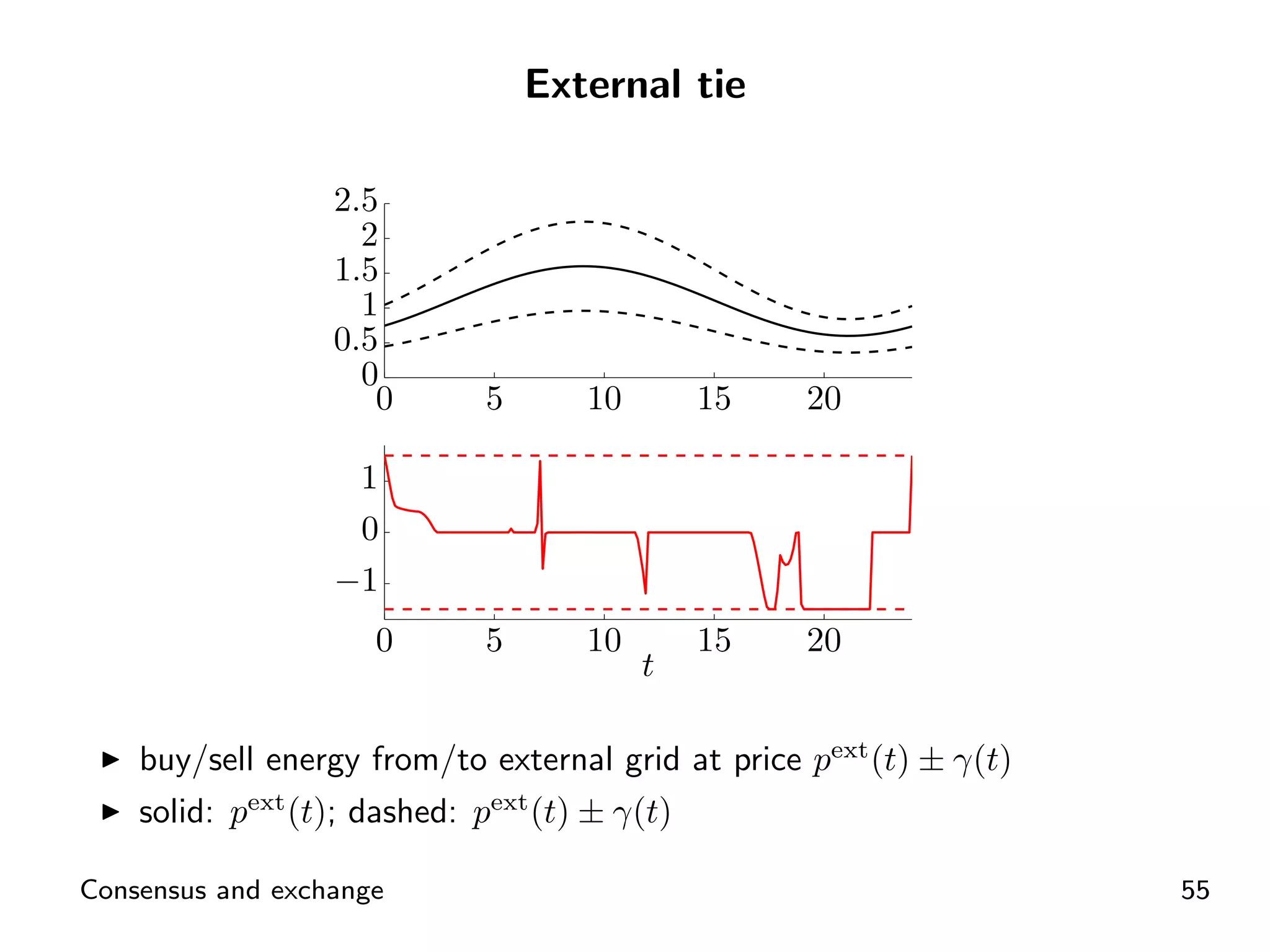
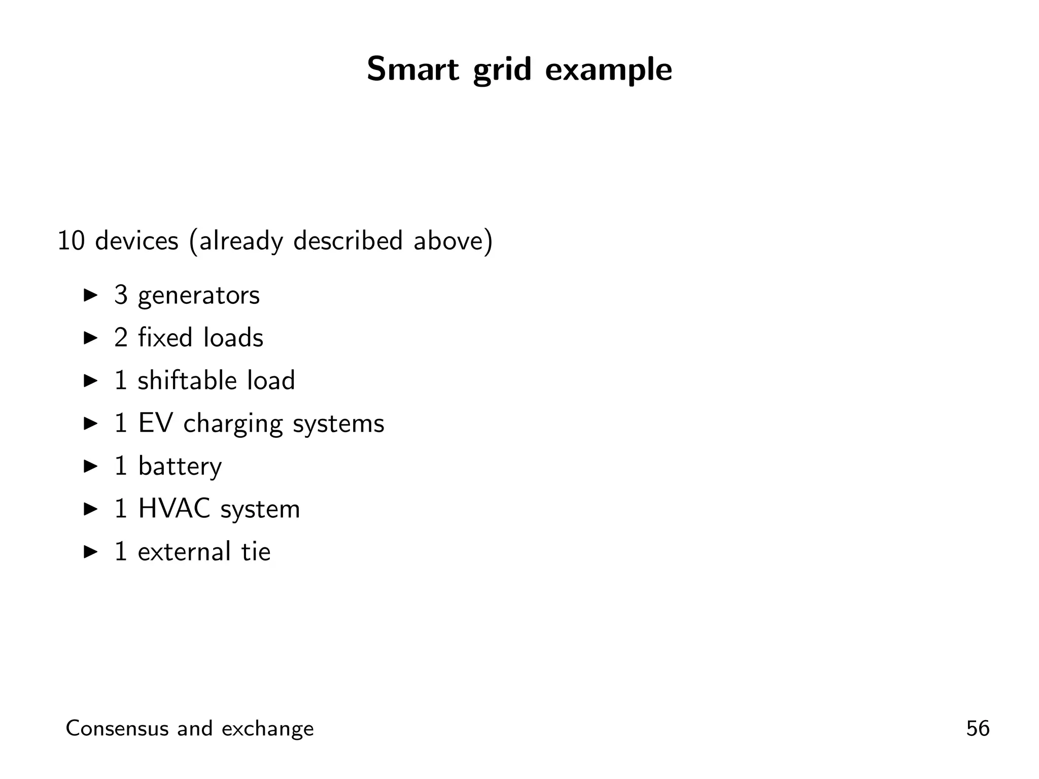
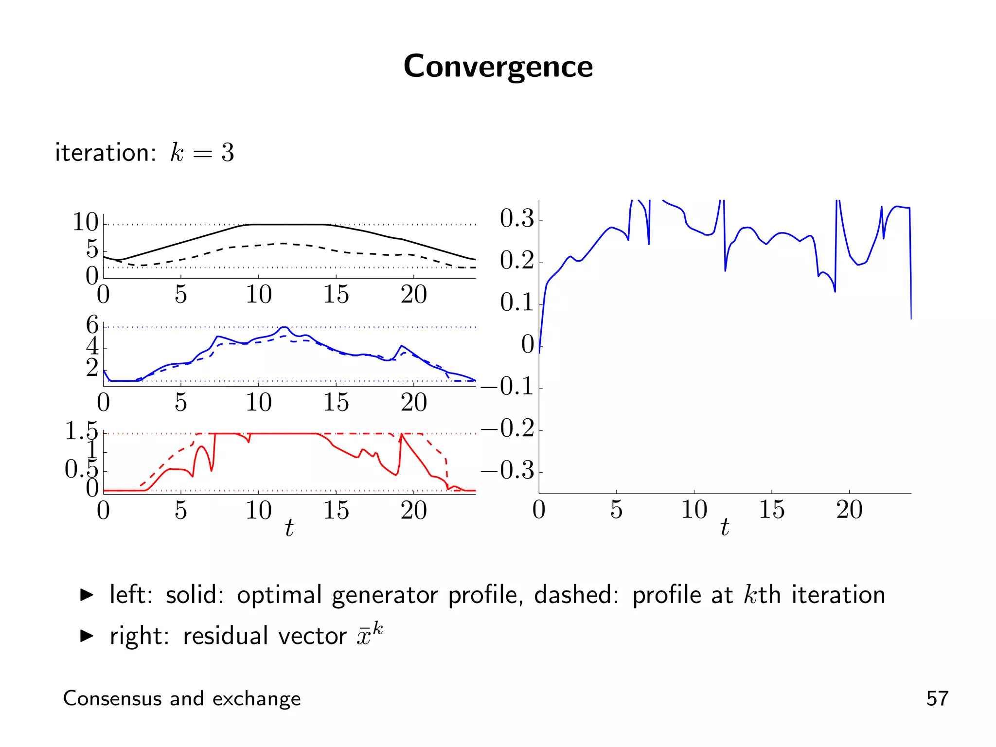
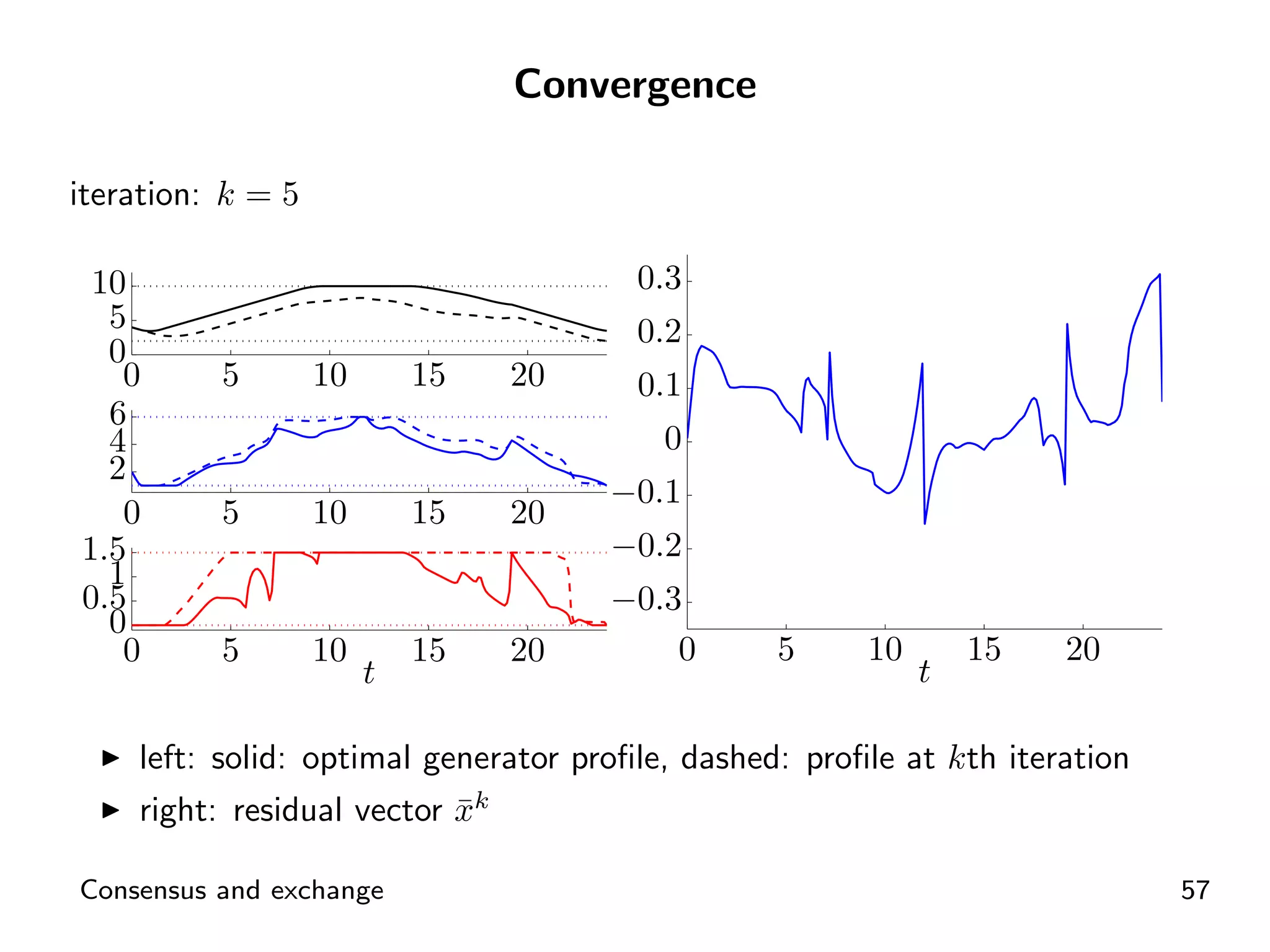
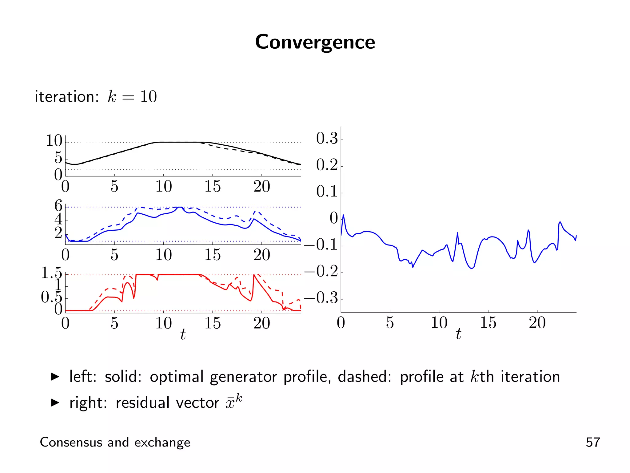
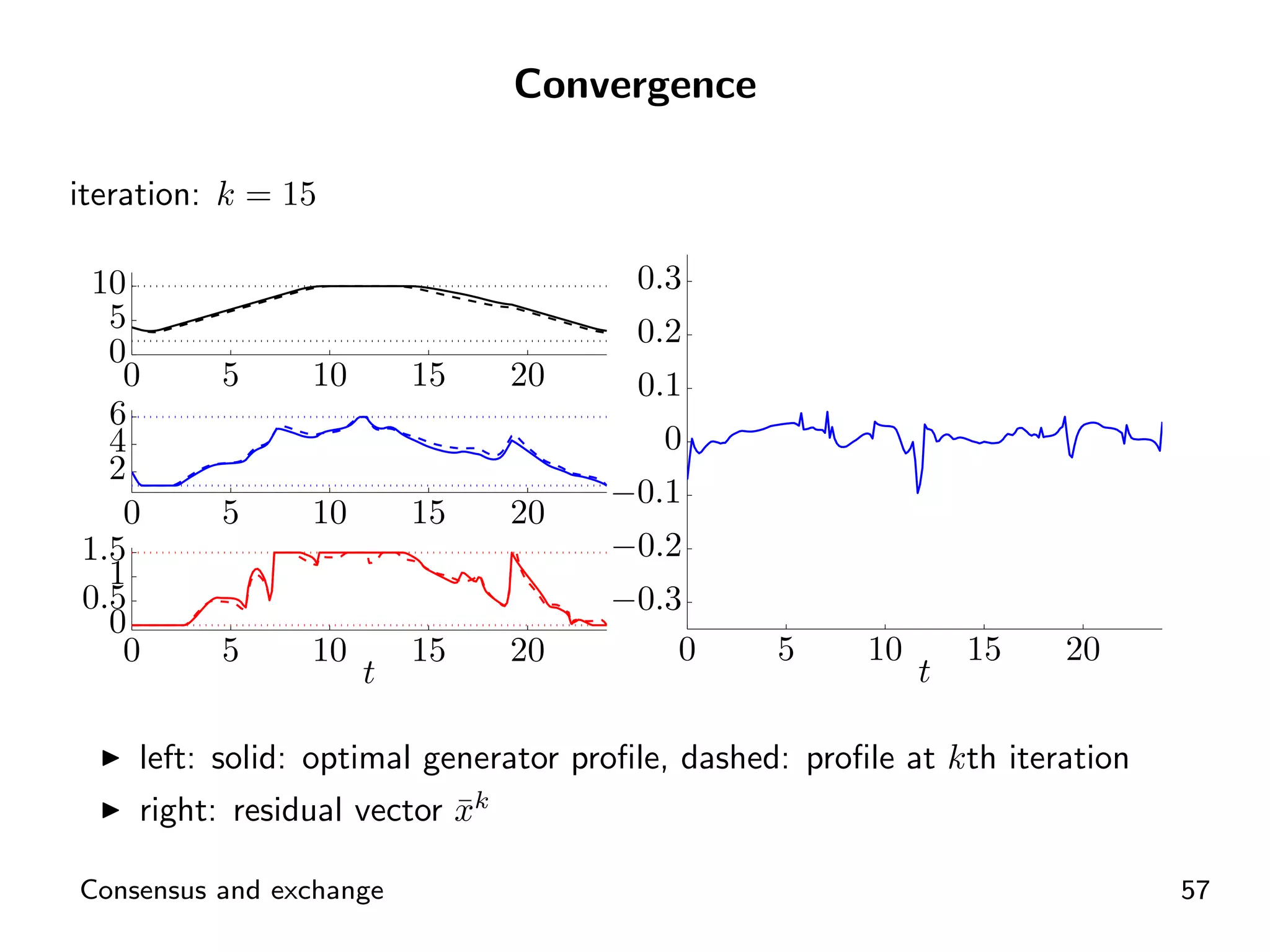
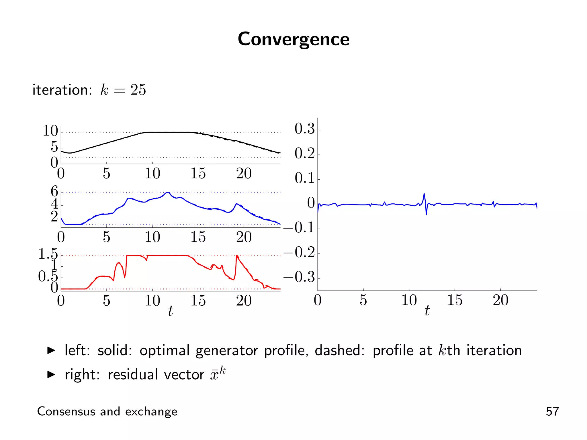
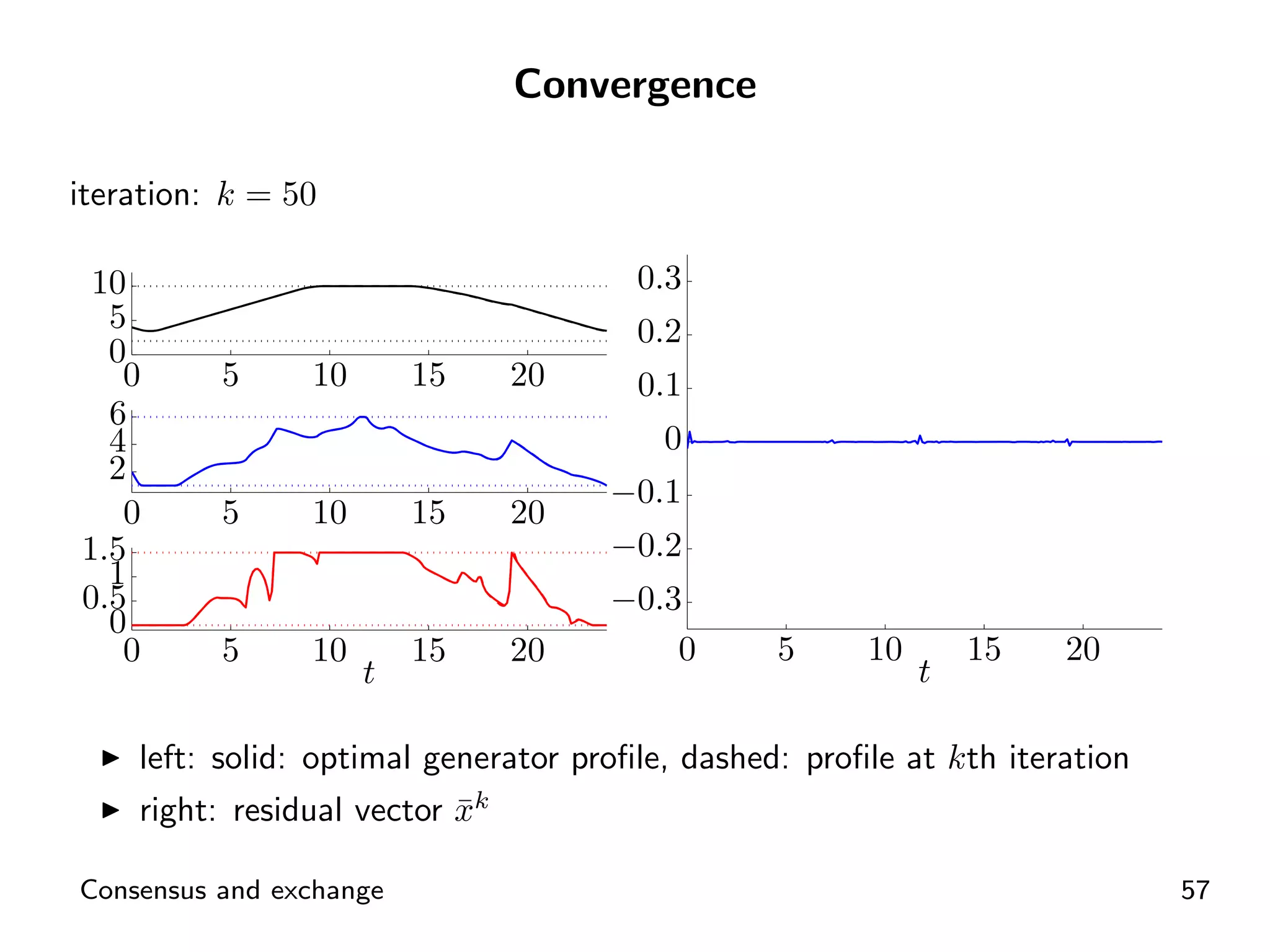
ADMM application for distributed energy exchange and management in devices.
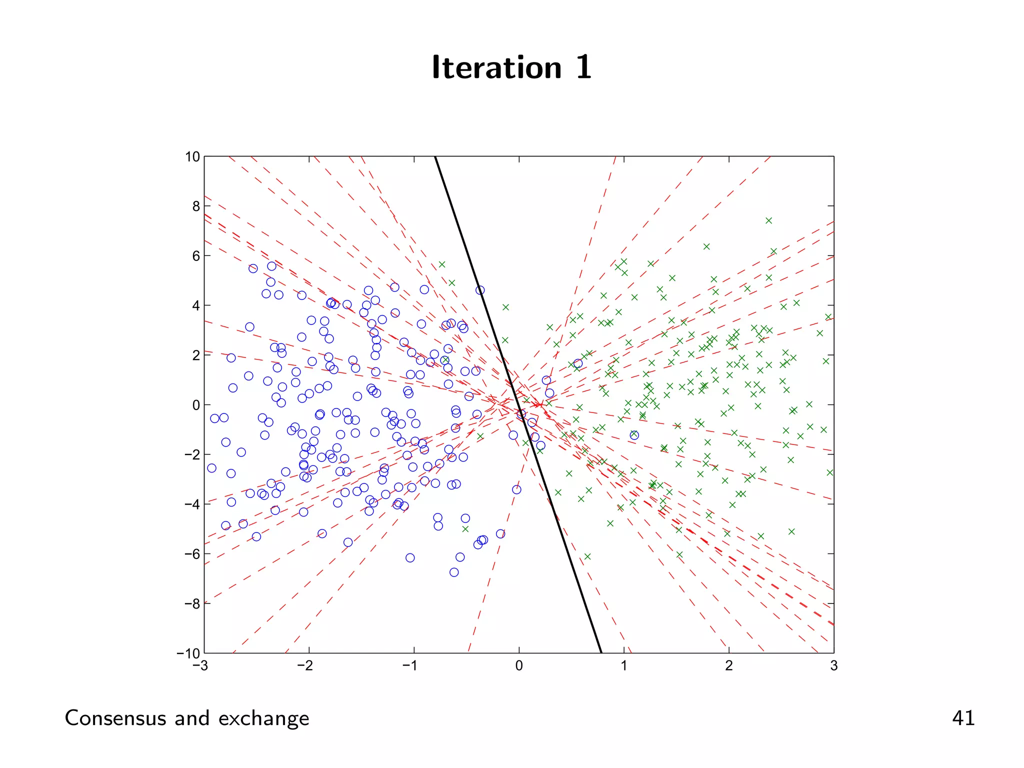
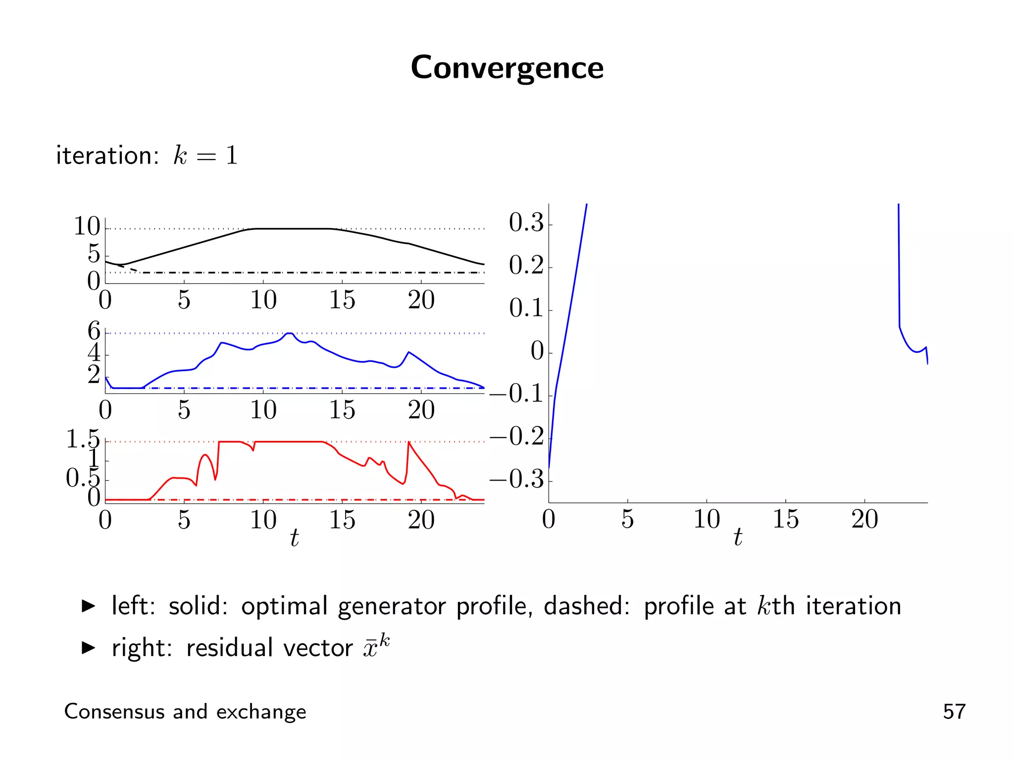
Visual representation of convergence behavior through multiple iterative activations.
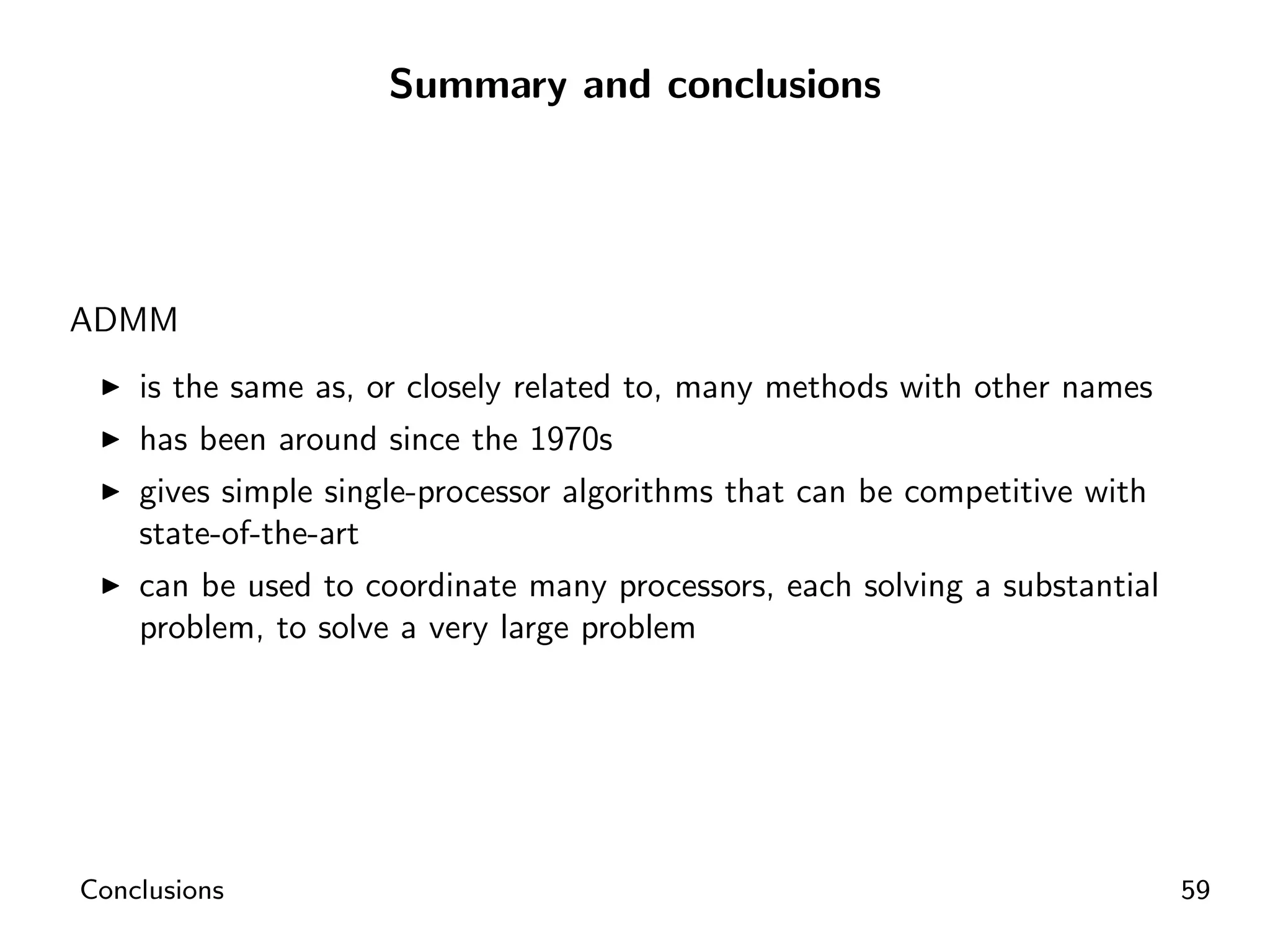
Summary of ADMM's relation to various optimization methods and efficiency in practice.