Concepts de base de la dynamique avion

1. Stability and Control
Introduction
An important concept that must be considered when designing an aircraft, missile , or
other type of vehicle, is that of stability and control. The study of stability is related to the flying
qualities of the vehicle and gives us some indication if the vehicle will be easy, difficult, or
impossible to fly. The control aspect of the study will indicate if the control surfaces are large
enough to force the vehicle into the desired flight maneuvers. Furthermore, if they are, can the
pilot provide the force necessary to move them of will s/he need some kind of assistance. Here
we will look at these problems, along with some others, as they pertain to aircraft, missiles, and
other vehicles.
The study of vehicle motion can be broken down into several different aspects. Although
complete studies require the investigations of all aspects simultaneously, a considerable amount
of information can be obtained from investigating one aspect at a time. In order to do these
studies it is necessary to introduce a mathematical model that serves to describe the system of
interest. It is in these mathematical models that the restrictive assumptions take place. To study
the complete problem of vehicle motion, we generally need the following sets of equations:
1. Force equations - Relate the motion of the center-of-mass to external forces.
2. Moment equations - Relate the rotation of the vehicle about the center-of-mass to the
external moments.
3. Elastic equations - Relate the deformations of the structure to the external forces and
moments and the loading imposed on it.
Under certain assumptions, we can study the above equations separately and relate these studies
to some topic in the general area of flight mechanics. In particular, the following subject areas
come to mind:
1. Force equations Vehicle performance
2. Moment equations Stability and control
3. Elastic equations Aeroelasticity, vibrations, and flutter
Consequently, this course will be predominately concerned with the moment equations. In order
to conduct such a study, it is necessary to introduce various axes systems in which to describe the
forces and moments.
Vehicle Axes Systems
Several axes systems are required to describe the motion of a vehicle. For now, however,
we will be interested only in axes systems who’s origin is fixed in the vehicle. In general these
axes systems are located such that the origin is at the center-of-mass (cm) of the vehicle. Several
different axes systems are defined, with the difference being related to their orientation in the
vehicle (or body). However, common to all axes systems used are the following: 1) the origin is

2. at the center-of-mass, 2) the x axis points forward, 3) the z axis points down (in the vehicle, i.e.
if the vehicle is upside down, the z axis would point up), and 4) the y axis points to the “right”
completing the right handed triad. The x-z plane generally corresponds to the vehicle plane of
symmetry. Typically the following body-fixed axes are used. Body-fixed axes are fixed in the
body (vehicle) with their origin at the center-of-mass and can be oriented as follows:
1. Principal Axes - aligned with the principal axes of the moments-of- inertia (0x pointing
generically forward, 0z pointing down, and 0y pointing out the right hand side). (Note the
principal axes are axes where all the products of inertia are equal to zero).
2. Water-Line (or sometimes called generic body-fixed axes) Axes - aligned with (or
parallel to) some arbitrary reference line in the vehicle (0x pointing forward, 0z pointing
down, and 0y completing the right hand set and pointing out the right hand side).
3. Stability Axes - The 0x axis is aligned with the relative wind’s projection onto the x-z
plane of symmetry in the reference flight condition, the oz axis is in the plane of
symmetry and points down, and the 0y axis completes the right hand set.
Once established, all axes systems remain fixed in the vehicle, rotating and translating with it.
Typical nomenclature used in describing motion along axes is as shown in the following table:
Axis Displacement Velocity Force Moment
linear angular linear angular
0x
(Longitudinal) x
bank(roll)*
surge
u p Fx, X L (K)**
0y
(Lateral) y
pitch*
sway
v q Fy, Y M
0z
(Normal) z
yaw*
heave
plunge
w
r Fz, Z N***
* The names bank (or roll), pitch, and yaw are not quite correct here. They are the names of these
motions if all the other angles are zero. For example, corresponds to a motion in pitch if and
are zero. Details will be uncovered much later in this course.
**K is used in the ocean vehicle description of roll moment. The aircraft folks have to carefully
distinguish between the roll moment (L) and the lift force (L)!
***N is also used for the normal force, the force along the 0z axis. Generally the normal force is
used when describing supersonic flow.

3. The standard right-hand convention is used to determine the signs of the angular
displacements, rates, and moments. If you put your right thumb in the direction of the axis of
interest, the fingers will curl in the direction of positive motion or moment. Using this
convention, we have the following:
, q, M positive nose up , r, N positive nose right (looking from the pilots
view point
, p, L positive right wing down
As indicated previously, there generally exists a plane of symmetry in the vehicle that
contains the x-z plane for all coordinate systems. Motions that are in this plane (that is, those
motions that do not cause the plane to translate sideways or to change its angular orientation) are
called symmetric motions. Motions that involve a rotation of the plane of symmetry or a
translation perpendicular to the plane of symmetry are called asymmetric motion. In addition,
forces and moments that would normally cause such motions are designated as symmetric and
asymmetric forces and moments. As a result, we can divide the forces and moments into two
groups as follows:
Longitudinal or symmetric group Lateral- directional or
asymmetric group
Fx, X, Fz, Z Fy, Y
u,w v
M L, N
q p,r
Motions in the plane-of-symmetry include climb, glide, straight, straight and level, pull-ups,
pitch overs, loops, etc. and are called longitudinal motions. Motions out of the plane-of-symmetry
include rolls, turns, spins, etc. and are called asymmetric or lateral-directional motions.
In order to simplify some later analysis a couple of assumptions are often made. These
may be good assumptions ( a weak assumption) or not-so-good (a strong assumption). The
assumption is a follows:
Assumption: For small disturbances away from some reference flight condition no coupling
exists between longitudinal and lateral-directional groups of motion.
This assumption implies tht small changes in the longitudinal variables u,w, and q have
no effect on the laterl-directional forces and moments, and that small changes in the lateral-directional
variables v, p, r, have no effect on the longitudinal forces and moments. This latter
assumption ( lateral motion variables affecting the longitudinal forces and moments) is more
restrictive than the former one. However for small disturbances, this cross coupling is usually of
second order ( depends on the square of the variables).

4. Reference Flight Condition (RFC)
In several of the previous discussions, we mentioned a reference flight condition. Here we
will define it more precisely. I order to discuss stability it is necessary to introduce the concept of
a reverence flight condition (RFC). A reference flight condition is one where all the derivatives
pertaining to the description of the vehicle motion are zero. Such a flight condition is also
called a steady state reference flight condition. A special case of a steady state reference flight
condition is an equilibrium reference flight condition. A vehicle in an equilibrium reference
flight condition has no acceleration so that the sums of the applied moments and forces is zero.
Examples of equilibrium reference flight conditions are constant velocity level flight, and
constant velocity climbing or diving flight. Examples of steady state reference flight conditions
are all the above as well as flight in a horizontal turn. (Note that a horizontal turn is not really
steady state because the derivative of the heading (yaw) angle , is not zero. However, when
dealing with stability, the angle does not appear in any equation describing the motion of
interest and hence is considered ignorable. As a consequence we can modify the definition of a
steady state reference flight condition to include those cases where only the derivatives of
variables that are ignorable are allowed to be non-zero)
In most of the problems that we will be dealing with in this course the reference flight
condition will be an equilibrium RFC where the applied forces and moments sum to zero. Then
for an equilibrium RFC we have:
Equilibrium RFC
Stability
For the purposes of this course it is convenient to define two types of stability, static
stability and dynamic stability. Although we can be much more precise, the following two
definitions will suffice for discussing vehicle stability.
Static stability - A vehicle is said to be statically stable at a given reference flight condition if,
when displaced away from that reference flight condition, unbalanced forces and moments
caused by the disturbance act in a direction that tends to return the vehicle to the original
reference flight condition.
We can note that while at the RFC, the forces and moments sum to zero. On disturbing
the vehicle away from the RFC the forces and moments may no longer equal zero. The vehicle is
statically stable if these unbalanced forces and moments tend to oppose the disturbance. Note that
there is no requirement that the vehicle actually returns to the RFC for it to be statically stable!
This part is addressed in the next definition.

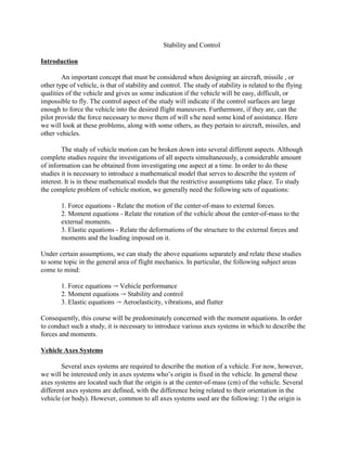
5. Dynamic stability - A vehicle is said to be dynamically stable at a given reference flight
condition if, when displace away from that reference flight condition that the disturbance goes to
zero as the time after the disturbance goes to infinity, that is the vehicle will indeed return to the
reference flight condition in time!
It should be clear to the casual observer that we require both static and dynamic stability for a
desirable aircraft. (When dealing with several degrees of freedom (longitudinal and lateral-directional)
it is possible to have a statically unstable vehicle that can be, within limits,
dynamically stable. An example is a spin stabilize rocket. For our purposes here and for most
aircraft we require both static and dynamic stability).
If we assume, for discussion purposes, that we can pin the aircraft at the center-of-mass in a wind
tunnel, and can set the controls so that the pitch moment is zero. This would be the reference
flight condition. Then we can disturb the aircraft by increasing the pitch angle, hold it, and then
let go. If the vehicle is statically stable, the moment caused by the displacement will be
oppose theta. Hence if theta is nose up (positive), then the moment will be nose down (negative).
Therefor on releasing the vehicle, the nose will start downward ( M = Iy ). If the vehicle is
dynamically stable, it will eventually reach equilibrium. An example of the motion of a vehicle
that is statically and dynamically stable is shown in the figure below.
Figure 1 A Static and Dynamically Stable Response to an Initial Displacement
An example of the response of a system that is statically stable and dynamically unstable
is given below. Here the vehicle is displace with a positive pitch angle. Since the system is
statically stable, the moment tends to oppose the positive displacement and when let go, the
system is pushed back towards the reference condition. However, it overshoots and tends to go
further in the wrong direction (all the while the moment continues to oppose the motion). This
type of behavior continues and the amplitude of the motion increases, causing the vehicle not to
return to the reference condition, therefore, dynamically unstable!

6. Figure 2 A Response for a System that is Statically Stable and Dynamically Unstable
A system that is statically unstable will just grow in amplitude after it is released from an
initial displacement. There will be no oscillation since there is no force or moment tending to
return the system to the reference state.
Aerodynamic Fundamentals
In order to determine static stability, we are interested in how the forces and moments due
to the surrounding fluid change with changes in the vehicle orientation or motion. These changes
are often related to the following dimensionless groups:
where = a force coefficient, = Mach number, and = Reynolds number. Also, = density
of fluid (air), = viscosity, a = speed of sound, V = speed of vehicle relative to the fluid, and
l = some characteristic length.
In general, dimensional analysis tells us that the force (and moment) coefficients are
functions of the other non-dimensional variables and take the form of:
Of particular interest in this course are the following coefficients:

7. Longitudinal
Lateral-Directional
where S = reference area = planform area of the wing of an aircraft
= cross section area for a missile
= length squared for a submarine
= longitudinal reference length
= mean aerodynamic chord for an aircraft
= diameter or length for a missile
= length for a submarine
b =lateral-directional reference length
= wing span for an aircraft
= diameter or length for a missile
= length for a submarine
We should also note the following in the coefficients above: 1) Force coefficients
generally use a capital letter in the subscript, lift coefficient CL. 2) Moment coefficients generally
use a lower case letter in the subscript, roll-moment coefficient Cl. There are exceptions to this
rule. Often times a 2-dimensional lift coefficient will use a lower case letter in the subscript.
Hence beware of how coefficients are defined. We can also note that different reference areas are
used for different vehicles. Consequently one can not in general compare the drag of two vehicles
by comparing their drag coefficients. Note also that for some vehicles the longitudinal reference
length and the lateral-directional reference length are the same, not so for an aircraft.
Since wings come in all shapes and sizes, and the chord length along the span of the wing
is usually not constant, it is convenient to define (loosely) an equivalent rectangular wing with a

8. constant chord length that has the same aerodynamic characteristics as the original wing,
particularly in pitch-moment characteristics. The chord of this “wing” is designated as the mean
aerodynamic chord, . A more complete discussion is presented in Appendix C of Etkin and
Reid, Dynamics of Flight. A detailed discussion of the mean aerodynamic chord is given in
Yates, A. H. “Notes on the Mean Aerodynamic Chord and the Mean Aerodynamic Centre of a
Wing,” J. Royal Aeronautical Society, Vol 56. P.461, June 1952.
Under certain circumstances (given in the above reference) the pitch moment
characteristics are the same for the rectangular “wing” and the actual wing if the mean
aerodynamic chord is calculated a certain way. That way now becomes the definition of the mean
aerodynamic chord for all wings. Hence we can calculate, if necessary, the mean aerodynamic
chord for any wing using the following relation:
This concludes the basic concepts section.