Downloaded 15 times


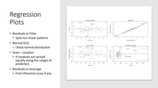
![# Read data
trainingSet <- read.csv(trainingFile, header = FALSE)
testSet <- read.csv(testFile, header = FALSE)
trainingSet$V65 <- factor(trainingSet$V65)
testSet$V65 <- factor(testSet$V65)
# Classify
library(caret)
knn.fit <- knn3(V65 ~ ., data=trainingSet, k=5)
# Predict new values
pred.test <- predict(knn.fit, testSet[,1:64], type="class")](https://image.slidesharecdn.com/rmachinelearning-171020072502/85/Clean-Learn-and-Visualise-data-with-R-18-320.jpg)
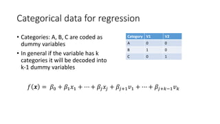
![# Confusion matrix
library(caret)
confusionMatrix(pred.test, testSet[,65])](https://image.slidesharecdn.com/rmachinelearning-171020072502/85/Clean-Learn-and-Visualise-data-with-R-19-320.jpg)
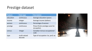
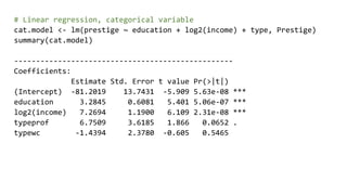
![# Pairs for the numeric data
pairs(Prestige[,-c(5,6)], pch=21, bg=Prestige$type)](https://image.slidesharecdn.com/rmachinelearning-171020072502/85/Clean-Learn-and-Visualise-data-with-R-24-320.jpg)
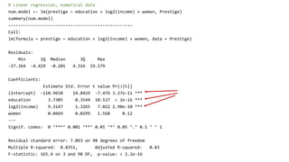
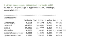
![# Pairs for the numeric data
cf <- et.fit$coefficients
ggplot(prestige, aes(education, prestige)) + geom_point(aes(col=type)) +
geom_abline(slope=cf[4], intercept = cf[1], colour='red') +
geom_abline(slope=cf[4] + cf[5], intercept = cf[1] + cf[2], colour='green') +
geom_abline(slope=cf[4] + cf[6], intercept = cf[1] + cf[3], colour='blue')](https://image.slidesharecdn.com/rmachinelearning-171020072502/85/Clean-Learn-and-Visualise-data-with-R-30-320.jpg)
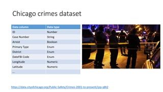
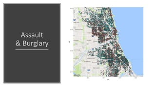
![# Read data
crimeData <- read.csv(crimeFilePath)
# Only data with location, only Assault or Burglary types
crimeData <- crimeData[
!is.na(crimeData$Latitude) & !is.na(crimeData$Longitude),]
selectedCrimes <- subset(crimeData,
Primary.Type %in% c(crimeTypes[2], crimeTypes[4]))
# Visualise
library(ggplot2)
library(ggmap)
# Get map from Google
map_g <- get_map(location=c(lon=mean(crimeData$Longitude, na.rm=TRUE), lat=mean(
crimeData$Latitude, na.rm=TRUE)), zoom = 11, maptype = "terrain", scale = 2)
ggmap(map_g) + geom_point(data = selectedCrimes, aes(x = Longitude, y = Latitude,
fill = Primary.Type, alpha = 0.8), size = 1, shape = 21) +
guides(fill=FALSE, alpha=FALSE, size=FALSE)](https://image.slidesharecdn.com/rmachinelearning-171020072502/85/Clean-Learn-and-Visualise-data-with-R-34-320.jpg)
![# k-means clustering (k=6)
clusterResult <- kmeans(selectedCrimes[, c('Longitude', 'Latitude')], 6)
# Get the clusters information
centers <- as.data.frame(clusterResult$centers)
clusterColours <- factor(clusterResult$cluster)
# Visualise
ggmap(map_g) +
geom_point(data = selectedCrimes, aes(x = Longitude, y = Latitude,
alpha = 0.8, color = clusterColours), size = 1) +
geom_point(data = centers, aes(x = Longitude, y = Latitude,
alpha = 0.8), size = 1.5) +
guides(fill=FALSE, alpha=FALSE, size=FALSE)](https://image.slidesharecdn.com/rmachinelearning-171020072502/85/Clean-Learn-and-Visualise-data-with-R-36-320.jpg)
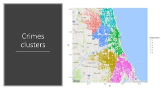
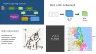

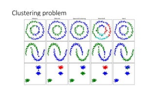
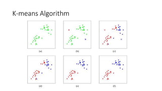
This document provides an overview of machine learning techniques using the R programming language. It discusses classification and regression using supervised learning algorithms like k-nearest neighbors and linear regression. It also covers unsupervised learning techniques including k-means clustering. Examples are presented on classification of movie genres, handwritten digit recognition, predicting occupational prestige, and clustering crimes in Chicago neighborhoods. Visualization methods are demonstrated for evaluating models and exploring patterns in the data.


![[GAN by Hung-yi Lee]Part 1: General introduction of GAN](https://cdn.slidesharecdn.com/ss_thumbnails/part1-180809095233-thumbnail.jpg?width=640&height=640&fit=bounds)


![제 23회 보아즈(BOAZ) 빅데이터 컨퍼런스 - [MBOAX] : ABSA를 활용한 소비자 반응 분석 기반 운영 효율화 대시보드 설계](https://cdn.slidesharecdn.com/ss_thumbnails/3-1boaz23rdconferencemboax-260203102709-9d519923-thumbnail.jpg?width=640&height=640&fit=bounds)


