qft practice calculation

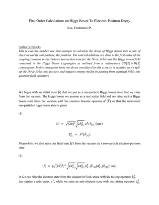
1. First Order Calculations on Higgs Boson To Electron-Positron Decay
Roa, Ferdinand J.P.
Author’s remarks
This is exercise number one that attempts to calculate the decay of Higgs Boson into a pair of
electron and its anti-particle, the positron. The said calculations are done to the first order of the
coupling constant in the Yukawa interaction term for the Dirac fields and the Higgs boson field
contained in the Higgs Boson Lagrangian as outlined from a rudimentary 𝑆𝑈(2) × 𝑈(1)
construction. In this interaction term, the decay considered in this exercise is manifest as we split
up the Dirac fields into positive and negative energy modes in passing from classical fields into
quantum field operators.
We begin with an initial state |𝑖⟩ that we put as a one-particle Higgs boson state that we raise
from the vacuum. The Higgs boson we assume as a real scalar field and we raise such a Higgs
boson state from the vacuum with the creation bosonic operator 𝑎†
(𝑘
⃗ ) so that the mentioned
one-particle Higgs boson state is given
(1)
|𝑖⟩ = √(2𝜋)3√2𝑃(1)
0
𝑎†
(𝑃
⃗(1))|𝑣𝑎𝑐⟩
𝑃(1)
0
= 𝑃0
(𝑃
⃗(1))
Meanwhile, we also raise our final state |𝑓⟩ from the vacuum as a two-particle electron-positron
state
(2)
|𝑓⟩ = (√(2𝜋)3)2
√2𝑘(1)
0
√2𝑘(2)
0
𝑏𝛼 ′
†
(𝑘
⃗ (2))𝑑𝛽 ′
†
(𝑘
⃗ (1))|𝑣𝑎𝑐⟩
In (2), we raise the electron state from the vacuum in Fock space with the raising operator 𝑏𝛼 ′
†
that carries a spin index 𝛼 ′, while we raise an anti-electron state with the raising operator 𝑑𝛽 ′
†

2. that also carries a spin index 𝛽 ′. These operators have anti-commutation relations that satisfy
those constructed for the Dirac (Fermion) fields.
Given (2), we then obtain its Hermitian adjoint
(3)
⟨𝑓| = ⟨𝑣𝑎𝑐|𝑑𝛽 ′(𝑘
⃗ (1))𝑏𝛼 ′(𝑘
⃗ (2))√2𝑘(2)
0
√2𝑘(1)
0
(√(2𝜋)3)2
With the application of the time evolution operator (teo) 𝑈(𝜏, 𝜏0) we evolve the initial state by
(4)
|𝑖⟩ → |𝜑⟩ = 𝑈(𝜏, 𝜏0)|𝑖⟩
We resort to Dyson expansion for our teo however we consider only first order expansion with
respect to the interaction coupling constant. This Dyson expansion is given by (in Heaviside
units)
(5)
𝑈(𝜏, 𝜏0) = 1 + ∑ (−𝑖)𝑞
∫ 𝑑𝑡1
𝜏
𝜏0
𝑛
𝑞 = 1
∫ 𝑑𝑡2
𝑡1
𝜏0
∫ 𝑑𝑡3
𝑡2
𝜏0
⋯ ∫ 𝑑𝑡𝑞
𝑡𝑞−1
𝜏0
𝐻
̂(𝑡1)𝐻
̂(𝑡2)𝐻
̂(𝑡3) ⋯ 𝐻
̂(𝑡𝑞)
where the Hamiltonian operators 𝐻
̂ are time ordered for all time intervals
(6)
𝑡𝑞 ≤ 𝑡𝑞−1 ≤ ⋯ ≤ 𝑡2 ≤ 𝑡1 ≤ 𝑡
In this exercise since we are dealing only with first order calculations we need not worry about
time ordering and to first order expansion we have
(7)
𝑈(𝜏, 𝜏0) = 1 − 𝑖 ∫ 𝑑𝑡
𝜏
𝜏0
𝐻
̂(𝑡)

3. The time evolution of our initial state is taken in the interaction picture so, the Hamiltonian
involved here is an interaction Hamiltonian that we take as that due to the interaction of the
Higgs boson and the Dirac fields. Thus,
(8)
𝐻
̂(𝑡) = 𝐻
̂𝑖𝑛𝑡(𝑡) = 𝑦 ∫ 𝑑3
𝑥 𝜓
̅
̂ (𝑥)𝜓
̂(𝑥) 𝜂̂(𝑥)
So to first order we write (7) as
(9)
𝑈(𝜏, 𝜏0) = 1 − 𝑖 𝑦 ∫ 𝑑4
𝑥 𝜓
̅
̂ (𝑥)𝜓
̂(𝑥) 𝜂̂(𝑥)
∫ 𝑑4
𝑥 = ∫ 𝑑𝑡
𝜏
𝜏0
∫ 𝑑3
𝑥
All the field operators contained in (9) can be split up into the positive and negative energy
modes that shall come later.
To the first order, we then write the matrix for this decay process as
(10)
⟨𝑓|𝑈(𝜏, 𝜏0)|𝑖⟩ = ⋯ − 𝑖𝑦 ⟨𝑓| ∫ 𝑑4
𝑥 𝜓
̅
̂ (𝑥)𝜓
̂(𝑥) 𝜂̂(𝑥)|𝑖⟩
We then proceed to split up the field operators into the positive and negative energy modes.
(To be continued…)
References
[1]Baal, P., A COURSE IN FIELD THEORY
[2]Cardy, J., Introduction to Quantum Field Theory
[3]Gaberdiel, M., Gehrmann-De Ridder, A., Quantum Field Theory
[4]Ashok Das, Lectures on Quantum Field Theory, World Scientific Publishing Co. Pte. Ltd., 27,
Warren Street, Suite 401-402, Hackensack, NJ 07601
[5]W. Hollik, Quantum field theory and the Standard Model, arXiv:1012.3883v1 [hep-ph]