11 construction productivity and cost estimation using artificial

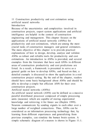
1. 11 Construction productivity and cost estimation using
artificial neural networks
Introduction
Because of the uncertainties and complexities involved in
construction projects, expert system applications and artificial
intelligence are helpful in the context of construction
engineering and management. This chapter focuses on the
applications of artificial neural networks (ANNs) for
productivity and cost estimations, which are among the most
crucial tasks of construction managers and general estimators.
The main objective of this chapter is to provide practical
explanations of how to design, develop, analyse and validate
ANNs as robust and reliable tools for productivity and cost
estimations. An introduction to ANNs is provided, and several
examples from the literature that have used ANNs in different
areas of construction productivity and cost predictions are
listed. As a result, a framework is presented to serve as a
general guide on how to develop ANNs, and based on that, a
detailed example is discussed to show the application in a real
construction project setting. By the end of the chapter, readers
should have some basic background about ANNs and should be
able to develop a simple but efficient ANN for their own
construction projects.
Artificial neural networks (ANNs)
An artificial neural network (ANN) can be defined as a massive
parallel distributed processor composed of simple processing
units (neurons) which are capable of storing experiential
knowledge and retrieving it for future use (Haykin 1999).
Neurons communicate by sending signals to each other over a
large number of weighted connections. Thus, ANNs can be
considered as an information processing technology that, by
learning from different experiences and generalizing from
previous examples, can simulate the human brain system. A
simple schematic diagram of a neuron is shown in Figure 11.1.

2. Figure 11.1 shows that each neuron has two distinct segments: a
summing junction that sums up the received inputs from
neighbours and an activation function that computes the output
signal, which is propagated to other neurons. The activation
function can be theoretically in any form such as signum, linear
or semilinear, hyperbolic tangent and sigmoid functions.
Figure 11.1 Schematic diagram of a neuron
To form a network, neurons are grouped into several layers,
namely input, hidden and output layers. Two types of network
topologies are shown in Figure 11.2:
· Feed-forward networks: data flows strictly from input to
output layers, and no feedback connections are allowed.
· Recurrent networks: feedback connections are allowed to
provide data flow from the following layers to the preceding
layers.
Figure 11.2 Different topologies of ANNs (Alavala 2006)
An ANN should be arranged in such a way that it can provide
the desired outputs for a set of inputs presented to the network.
To do so, either connection weights should be set using prior
knowledge or the network should be trained by training samples
(training sets). Connection weights are then updated based on
‘the learning rules’. There are two types of learning in ANNs:
· Supervised learning (associative learning): both input and
output training pairs are presented to the network, and the
network will learn based on the presented samples.
· Unsupervised learning (self-organization): there is no prior set
of categories to be presented to the network, and the system
develops its own representation of the input stimuli.
Almost all the learning rules are variants of the ‘Hebbian’
learning rule, which simply says that if two neurons are active,
their interconnection must be strengthened. Based on this
learning rule, the ‘delta rule’ uses the differences between
actual and desired activation for modifying the connection
weights.

3. Multilayer feed-forward neural networks (Figure 11.2) are the
most commonly used architecture in the engineering fields,
including construction engineering and management. The so-
called back-propagation learning algorithm (Rumelhart,
Hintont et al. 1986), which is a generalization of the delta rule,
is generally used in these types of networks. A set of training
samples is presented to the network, and based on the activation
functions of the hidden and output layers, the network outputs
are calculated, and are then compared with the actual (desir ed)
outputs. The error is calculated (i.e. the difference between the
actual and network output) and is propagated back to the
network, the connection weights are modified and this
procedure is repeated until the network reaches the stop
criterion.
Generalization is the ability of neural networks to produce
reasonable outputs for inputs for which they have not been
trained. Learning capabilities and generalization are among the
differences between ANNs and conventional models. ANNs are
also useful where the processes to be modelled are too complex
to be represented by analytical models. Based on the previous
examples, neural networks can be built to make new decisions,
classify new patterns and make forecasts and predictions. The
most important advantage of ANNs over conventional models
(mathematical and statistical) is their ability to adjust their
weights to optimize their behaviour in different situations
(Boussabaine 1996). Moreover, ANNs may include multiple
outputs simultaneously (e.g. cost and productivity are both
predictable using a single network providing the required inputs
are used) when compared to multiple regression analysis
(MRA), which can only estimate one output at a time.
Using ANNs for productivity and cost estimations
This section describes the procedure for the development of
simple but efficient ANNs for productivity and cost predictions.
Past studies are described and a framework established that
shows the steps required for the development of ANNs for
productivity and cost estimations. Based on that, an example is

4. provided to show the accuracy of such networks in the context
of real construction projects.
Suppose an estimator wants to predict the total construction cost
of a new high-rise building project for a general contractor. The
focus here is to describe the problem in such a way that it can
be solved by the predictive ability of an ANN. To do so, the
first step is to collect the factors (inputs) that affect the cost of
the project, which are mainly project specifications such as total
gross floor area, the type of building structure (steel or
concrete), specific resources required and the like. Note that the
main output is the total cost of the building. The estimator is
then required to look at the previous projects (similar proj ects
by the same contractor or other general contractors) to be used
as the training examples for the ANN. The next step is to
configure the network by choosing the number of layers, type of
activation functions for hidden and output layers and number of
neurons in each layer. These configurations are usually
determined by trial and error. It has been shown that one layer
of hidden units is enough to approximate any function to an
arbitrary level of precision (Alavala 2006), but there is no
specific rule regarding the number of neurons in the hidden
layer.
There are several commercial packages available for design and
analysis of ANNs. Most of them have graphical interfaces and
can be used as add-ins for commonly used spreadsheet programs
like Microsoft Excel. After the network is developed and
trained, it is ready to be used for estimation purposes in the new
projects with acceptable accuracy considering the uncertainties
involved in the construction industry. A similar procedure can
be used to estimate the productivity of different construction
operations.
The following are some examples from the literature that have
used the same method to develop ANNs for productivity and
cost estimation of different construction projects. Some of the
following examples have used other learning algorithms, but the
procedure to develop the ANNs is more or less the same.

5. ANNs for total cost and duration estimations
One of the most important tasks for the construction
management team is to provide cost and schedule estimations
for different construction projects. Because of the predictive
capabilities of ANNs, they have been widely used to provide
more accurate cost and schedule predictions when compared to
conventional estimation methods. This can result in fewer cases
of cost overruns and fewer schedule discrepancies during the
construction phase. Some of the examples in this area included
predicting:
· highway and road tunnel construction costs (Hegazy and Ayed
1998; Wilmot and Mei 2005; Wichan et al. 2009; Petrousatou et
al. 2011)
· duration of reconstruction projects and the related costs
(Attalla and Hegazy 2003; Chen and Huang 2006)
· total cost and construction duration of residential buildings
(Bhokha and Ogunlana 1999; Emsley et al. 2002; Kim et
al. 2004)
· cost of structural systems of buildings (Günaydın and Doğan
2004)
· cost indices and unit price analysis (Baalousha and Çelik
2011).
The list shows that ANNs can be applied at any level for cost
and duration estimations, from unit price analysis, which is the
basis of cost predictions, to overall cost estimations of different
construction projects including infrastructure and residential
buildings.
ANNs for productivity modelling and estimation
Another vital task in the construction management field is to
provide productivity rates and measurement, especially in areas
such as resource allocation and management, scheduling,
estimating, accounting, cost control and payroll (Herbsman and
Ellis 1990). Contractors should have reliable estimates for
different construction operations which are needed for planning
and scheduling purposes. ANNs can be utilized in this area as a
robust tool for productivity modelling and estimation. Some of

6. the construction processes and operations for which ANNs have
been used to model productivity are:
· concrete pouring, formwork and finishing tasks (Portas and
AbouRizk 1997; Ezeldin and Sharara 2006; Dikmen and Sonmez
2011)
· hoisting times (hook times) of tower cranes (Tam et al. 2004)
· pile construction (Zayed and Halpin 2005)
· plastering activities (Oral et al. 2012)
· earth-moving equipment (Chanda and Gardiner 2010; Hola and
Schabowicz 2010; Han et al. 2011).
Most of these studies show the application of ANNs for
productivity modelling at the task level. ANNs are, however,
applicable to any level of productivity prediction just as they
can be applied to various levels of cost estimation.
Based on the previous studies, Figure 11.3 depicts a framework
that shows all of the steps required to develop efficient ANNs
for productivity and cost estimation.
Example: estimating on-site productivity of precast installation
activities
Problem formulation
A contractor in charge of the installation of different precast
elements wanted to have more accurate estimates of on-site
erection activities in order to manage the required resources
more efficiently. An estimator was hired to provide a tool which
could predict the time needed to install different precast
components such as walls, columns, beams and slabs. For better
understanding of the problem requirements, several preliminary
site visits were conducted, and the estimator determined that a
typical erection process or cycle includes several activities and
resources; these are shown graphically in Figure 11.4.
Figure 11.3 A framework for the development of an ANN for
productivity and cost estimation
Factors affecting productivity of precast installation
Based on Figure 11.4 and through site visits, expert interviews
and a literature review, the following factors were identified as

7. being important for productivity of precast erection processes:
· Weight: component weight (tonnes)
· Area: the largest surface area of the element (m2)
· Length: the longest dimension of the element (m)
· Height: component height (m)
· Storage type: the component is stored among others or isolated
(0: isolated; 1: among others)
· Storage to crane: distance from the element to the centre of
the crane at the storage area (m)
· Installation to crane: distance from the installation point to the
centre of the crane (m)
· Crane angle: angular movement of crane (degrees)
· Installation type: the component is installed among others or
isolated (0: isolated; 1: among others)
· Location type: the component is part of the exterior or interior
(0: interior; 1: exterior)
· Elevation: elevation of the installation point (m).
Figure 11.4 Precast installation activities (Najafi and Tiong
2012)
Other factors such as weather conditions, management
conditions, crew skill and the like could also be considered;
however, for simplicity, they were not included in this example.
Data collection
The next step was to collect the required data needed for ANN
training and validation. In this case, the estimator collected the
data regarding the installation of 91 precast elements (walls,
columns and slabs) through site observations. General
specifications of the collected data are shown in Table 11.1.
Table 11.1 shows that the observed precast components are
among the typical elements that are widely used in construction
projects. The results of the study can therefore be generalized
and applied to new projects as well.
Selecting the ANN architecture and training algorithm
The estimator then used a commercial package (e.g. Neuro

8. Solution
sTM) to design the ANN. For simplicity, a typical feed-forward
back-propagation network was chosen as the main architecture.
The inputs of the network were the factors described in the
previous sections, and the main output is the total installation
time in minutes.
Table 11.1 General specifications of the collected data
From 91 observations, 60 data points were randomly selected
for the training of the network, 16 cases for cross-validation,
and the remaining 15 data points were used for validation
purposes. Use of the cross-validation technique ensures that the
network is not overtrained (a situation in which the network
performs well on the training set but performs poorly on the test
data). With this method, the stop criterion is chosen in such a
way that as soon as the error in the cross-validation set starts to
increase, the training will be stopped. Since there is no specific
rule for the configuration of ANNs, the estimator should
develop several ANNs and choose the one with minimum error.
Table 11.2 shows different ANN architectures and the
corresponding mean squared error (MSE) and mean absolute
error (MAE), which are calculated using the following

9. formulae:
YNN is the network output and YA is the actual (desired)
output for each testing data point. The best-performing network,
the one that contains the minimum error (min. MSE), is
highlighted. Note that in Table 11.2, architecture 11–7–1
denotes a network with three layers (one hidden layer)
containing 11, 7 and 1 neurons in the input, hidden, and output
layers, respectively.
Validation and performance of the selected model
A set of 15 data points was used to test the performance of the
model against the actual data collected from the construction
sites, and the results are shown in Figure 11.5.
Table 11.2 Selection of the best performing network
Figure 11.5 Predicted vs. actual installation times
The mean absolute percentage error (MAPE) calculated
by Equation 11.3 was equal to 19.86%, which means that the
installation times predicted by the ANN are about 20% higher or
lower than the actual installation times, which can be
considered to be an acceptable performance considering the
uncertainties involved in construction estimations.

10. different construction projects. The main differences are in the
factors affecting productivity or cost estimations and the
procedure followed to collect the required data. It should be
noted that the aforementioned errors can be further minimized
by increasing the sample size of the collected data (training
set). Additionally, the use of other network types with different
learning algorithms may result in better estimates. Statistical
tests and analysis are also recommended for further comparison
between the characteristics of the actual data and the estimated
data provided by ANNs.
Hybrid use of artificial intelligence
The performance of ANNs can be further enhanced when they
are used together with other artificial intelligence techniques
such as fuzzy logic and genetic algorithms. Basically, fuzzy and
neural systems are structurally different; however, they share a
complementary nature and can be integrated to improve the
overall flexibility and expressiveness of neural networks
(Tsoukalas and Uhrig 1997). ANNs can be applied in function
approximation, pattern recognition and automatic learning. On
the other hand, fuzzy logic is efficient in modelling
uncertainties. Their combination is therefore useful in dealing
with certain construction management research problems that
require accurate approximation while including different types

11. of uncertainties. The performance of ‘neurofuzzy’ systems can
be further improved by using genetic algorithms (Holland 1992)
to optimize ANN parameters such as connection weights or
network topologies (number of neurons in the hidden layer).
Additionally, with the increasing adoption of building
information modelling (BIM) packages, there is a need to
develop ANN analysis as a separate module that can be
integrated with BIM systems. Architects, engineers, contractors
and owners use BIM programs to plan, collaborate and predict
performance before breaking ground on buildings. This chapter
shows that ANNs are able to provide accurate productivity
modelling of any construction operation, and the integration of
ANNs with BIM systems is beneficial for both tools. This can
be shown by the example of precast installation. Note that to
use ANNs to estimate the installation time of each precast
element, an estimator should manually feed all of the required
input data such as element weight, surface area, the longest
length and so on, as these are the factors affecting productivity
in precast installation. Since most of this data is already
available in the BIM model of the building, a computer program
can be developed to automatically extract the required input for
ANNs from the BIM system and perform the analysis. The
results from ANNs can be then linked back to the BIM system
to predict the performance more accurately.
Conclusions

12. Artificial neural networks are an information-processing
technology that simulates the human brain system through
learning from different experiences and generalizing from
previous examples. Since the 1990s, this technique has been
widely used in various areas of construction engineering and
management, including cost and project duration estimations,
bidding models and mark-up estimations, productivity
modelling, prequalification of contractors and risk management.
This chapter summarized how ANNs can be easily applied to the
two most important construction management tasks, cost
estimation and productivity modelling. The procedures for using
ANNs in other areas are similar to those depicted in the
framework described here.
Some construction management problems deal with different
levels of uncertainty. In these cases, the use of ‘neurofuzzy’
systems is highly recommended to add the flexibility required to
solve these problems with the integration of ANNs with fuzzy
systems. Additionally, by increasing adoption of BIM packages,
the integration of BIM systems with ANNs is suggested in order
to automate the data entry process as well as to improve the
accuracy of performance prediction in the BIM system.
Finally, it is recommended that construction management
research scholars and industry players further investigate the
applications of ANNs. There are several commercial and open-
source packages that provide user-friendly interfaces which can

13. be easily used to develop efficient ANNs with only basic
knowledge of this technique. Although ANNs have been used
for more than two decades in the construction industry, further
research gaps can be identified through extensive literature
review, especially in those areas where ANNs have been
utilized in other industries.