TTT,CCT curves,FAtigue

1. 1) Write Avrami rate equation in phase transformation.
The Avrami equation describes how solids transform from one phase (state of matter) to
another at constant temperature. It can specifically describe the kinetics of crystallisation., can be
applied generally to other changes of phase in materials, like chemical reaction rates, and can even
be meaningful in analyses of ecological systems.
2) List the different phases that exist in Fe-C equilibrium diagram.
shows the equilibrium diagram for combinations of carbon in a solid solution of iron. The
diagram shows iron and carbons combined to form Fe-Fe3C at the 6.67%C end of the diagram. The
left side of the diagram is pure iron combined with carbon, resulting in steel alloys. Three
significant regions can be made relative to the steel portion of the diagram. They are the eutectoid
E, the hypoeutectoid A, and the hypereutectoid B. The right side of the pure iron line is carbon in
combination with various forms of iron called alpha iron (ferrite), gamma iron (austenite), and
delta iron. The black dots mark clickable sections of the diagram.
Allotropic changes take place when there is a change in crystal lattice structure. From 2802º-2552ºF
the delta iron has a body-centered cubic lattice structure. At 2552ºF, the lattice changes from a
body-centered cubic to a face-centered cubic lattice type. At 1400ºF, the curve shows a plateau but
this does not signify an allotropic change. It is called the Curie temperature, where the metal
changes its magnetic properties.
Two very important phase changes take place at 0.83%C and at 4.3% C. At 0.83%C, the
transformation is eutectoid, called pearlite.
gamma (austenite) --> alpha + Fe3C (cementite)
At 4.3% C and 2066ºF, the transformation is eutectic, called ledeburite.
L(liquid) --> gamma (austenite) + Fe3C (cementite)
3.What is a fatigue fracture?
The majority of engineering failures are caused by fatigue. Fatigue failure is defined as the
tendency of a material to fracture by means of progressive brittle cracking under repeated
alternating or cyclic stresses of an intensity considerably below the normal strength. Although the
fracture is of a brittle type, it may take some time to propagate, depending on both the intensity and
frequency of the stress cycles.
4) What is a composite material?
A composite material (also called a composition material or shortened to composite) is a
material made from two or more constituent materials with significantly different physical or
chemical propertie that, when combined, produce a material with characteristics different from thes

2. individual components. The individual components remain separate and distinct within the finished
structure. The new material may be preferred for many reasons: common examples include
materials which are stronger, lighter, or less expensive when compared to traditional materials.
More recently, researchers have also begun to actively include sensing, actuation, computation and
communication into composites,which are known as robotic materials.
5) What are the coordinates of a phase diagram?
pressure (P) and temperature (T) are usually the coordinates. The phase diagrams usually
shows the (P, T) conditions for stable phases.
6.What is the abbreviation of TTT diagram?
Time temperature transformation
7.What is diffusion?
Diffusion is the net movement of molecules or atoms from a region of high concentration to a
region of low concentration
8.What is an interstitial impurity?
Small impurity interstitial atoms are usually on true off-lattice sites between the lattice atoms.
Such sites can be characterized by the symmetry of the interstitial atom position with respect to its
nearest lattice atoms
For instance, an impurity atom I with 4 nearest lattice atom A neighbours (at equal
distances) in a FCC lattice is in a tetrahedral symmetry position, and thus can be called a tetrahedral
interstitial.
9.What is a brittle facture?
Brittle fracture is the fracture of a metal or other material without appreciable prior plastic
deformation. It is a break in a brittle piece of metal which failed because stress exceeded cohesion.
Brittle fracture of normally ductile steels occurs primarily in large, continuous, box-like structures .
10. What is hardness?
Hardness is a measure of how resistant solid matter is to various kinds of permanent shape change
when a compressive force is applied. Some materials, such as metal, are harder than others.
Macroscopic hardness is generally characterized by strong intermolecular bonds, but the behavior
of solid materials under force is complex; therefore, there are different measurements of hardness:
scratch hardness, indentation hardness, and rebound hardness.
11.Define ceramics.
A ceramic is an inorganic non-metallic solid made up of either metal or non-metal compounds
that have been shaped and then hardened by heating to high temperatures. In general, they are hard,
corrosion-resistant and brittle.
Ceramic comes from the Greek word meaning ‘pottery’. The clay-based domestic wares, art objects

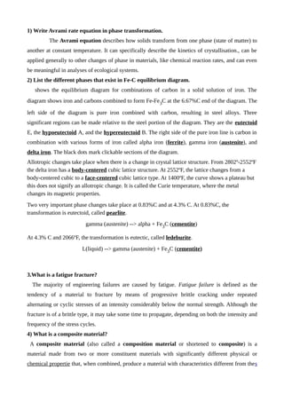
3. and building products are familiar to us all, but pottery is just one part of the ceramic world.
12.How are polymers classified?
A))based on synthesis
B))based on inter molecular forces
C))from source
D))based on material
E))based on structure
*Draw and explain Fe-Fe3C phase diagram?
A study of the microstructure of all steels usually starts with the iron carbide . It provides an
invaluable foundation on which to build knowledge of both carbon steels and alloy steels, as well
as a number of various heat treatments they are usually subjected to (hardening, annealing, etc).
Figure 1. The Fe-Fe3C phase diagram shows which phases are to be expected at metastable
equilibrium for different combinations of carbon content and temperature. The metastable Fe-C
phase diagram was calculated with cal , coupled with PBIN thermodynamic database.
At the low-carbon end of the Fe-Fe3C phase diagram, we distinguish ferrite (alpha-iron), which
can at most dissolve 0.028 wt. % C at 738 °C, and austenite (gamma-iron), which can dissolve 2.08
wt. % C at 1154 °C. The much larger phase field of gamma-iron (austenite) compared with that of

4. alpha-iron (ferrite) indicates clearly the considerably grater solubility of carbon in gamma-iron
(austenite), the maximum value being 2.08 wt. % at 1154 °C. The hardening of carbon steels, as
well as many alloy steels, is based on this difference in the solubility of carbon in alpha-iron
(ferrite) and gamma-iron (austenite).
At the carbon-rich side of the metastable Fe-C phase diagram we find cementite (Fe3C). Of less
interest, except for highly alloyed steels, is the delta-ferrite at the highest temperatures.
The vast majority of steels rely on just two allotropes of iron: (1) alpha-iron, which is body-
centered cubic (BCC) ferrite, and (2) gamma-iron, which is face-centered cubic (FCC) austenite.
At ambient pressure, BCC ferrite is stable from all temperatures up to 912 °C (the A3 point), when
it transforms into FCC austenite. It reverts to ferrite at 1394 °C (the A4 point). This high-
temperature ferrite is labeled delta-iron, even though its crystal structure is identical to that of
alpha-ferrite. The delta-ferrite remains stable until it melts at 1538 °C.
Regions with mixtures of two phases (such as ferrite + cementite, austenite + cementite, and ferrite
+ austenite) are found between the single-phase fields. At the highest temperatures, the liquid phase
field can be found, and below this are the two-phase fields (liquid + austenite, liquid + cementite,
and liquid + delta-ferrite). In heat treating of steels, the liquid phase is always avoided.
The steel portion of the Fe-C phase diagram covers the range between 0 and 2.08 wt. % C. The cast
iron portion of the Fe-C phase diagram covers the range between 2.08 and 6.67 wt. % C.
The steel portion of the metastable Fe-C phase diagram can be subdivided into three regions:
hypoeutectoid (0 < wt. % C < 0.68 wt. %), eutectoid (C = 0.68 wt. %), and hypereutectoid (0.68
< wt. % C < 2.08 wt. %).
A very important phase change in the Fe-Fe3C phase diagram occurs at 0.68 wt. % C. The
transformation is eutectoid, and its product is called pearlite (ferrite + cementite):
gamma-iron (austenite) —> alpha-iron (ferrite) + Fe3C (cementite).
Some important boundaries at single-phase fields have been given special names. These include:
• A1 — The so-called eutectoid temperature, which is the minimum temperature for austenite.
• A3 — The lower-temperature boundary of the austenite region at low carbon contents; i.e., the
gamma / gamma + ferrite boundary.
• Acm — The counterpart boundary for high-carbon contents; i.e., the gamma / gamma + Fe3C
boundary.
Sometimes the letters c, e, or r are included:

5. • Accm — In hypereutectoid steel, the temperature at which the solution of cementite in austenite is
completed during heating.
• Ac1 — The temperature at which austenite begins to form during heating, with the c being derived
from the French chauffant.
• Ac3 — The temperature at which transformation of ferrite to austenite is completed during
heating.
• Aecm, Ae1, Ae3 — The temperatures of phase changes at equilibrium.
• Arcm — In hypereutectoid steel, the temperature at which precipitation of cementite starts during
cooling, with the r being derived from the French refroidissant.
• Ar1 — The temperature at which transformation of austenite to ferrite or to ferrite plus cementite
is completed during cooling.
• Ar3 — The temperature at which austenite begins to transform to ferrite during cooling.
• Ar4 — The temperature at which delta-ferrite transforms to austenite during cooling.
If alloying elements are added to an iron-carbon alloy (steel), the position of the A1, A3, and Acm
boundaries, as well as the eutectoid composition, are changed. In general, the austenite-stabilizing
elements (e.g., nickel, manganese, nitrogen, copper, etc) decrease the A1 temperature, whereas the
ferrite-stabilizing elements (e.g., chromium, silicon, aluminum, titanium, vanadium, niobium,
molybdenum, tungsten, etc) increase the A1 temperature.
The carbon content at which the minimum austenite temperature is attained is called the eutectoid
carbon content (0.68 wt. % C in case of the Fe-Fe3C phase diagram). The ferrite-cementite phase
mixture of this composition formed during slow cooling has a characteristic appearance and is
called pearlite and can be treated as a microstructural entity or microconstituent. It is an aggregate
of alternating ferrite and cementite lamellae that coarsens (or "spheroidizes") into cementite
particles dispersed within a ferrite matrix after extended holding at a temperature close to A1.
Finally, we have the martensite start temperature, Ms, and the martensite finish temperature,
Mf:
• Ms — The highest temperature at which transformation of austenite to martensite starts during
rapid cooling.
• Mf — The temperature at which martensite formation finishes during rapid cooling.
*Explain how Tensile Test is conducted. What property is studied and how?
Tensile Test Experiment
Introduction
One material property that is widely used and recognized is the strength of a material. But what

6. does the word “strength” mean? “Strength” can have many meanings, so let us take a closer look at
what is meant by the strength of a material. We will look at a very easy experiment that provides
lots of information about the strength or the mechanical behavior of a material, called the tensile
test.
The basic idea of a tensile test is to place a sample of a material between two fixtures called “grips”
which clamp the material. The material has known dimensions, like length and cross-sectional area.
We then begin to apply weight to the material gripped at one end while the other end is fixed. We
keep increasing the weight (often called the load or force) while at the same time measuring the
change in length of the sample.
Tensile Test
One can do a very simplified test at home.
If you have a way to hang one end of some material from a solid point that does not move, then you
can hang weights on the other end.
Measure the change in length while adding weight until the part begins to stretch and finally breaks.
The result of this test is a graph of load (amount of weight) versus displacement (amount it
stretched). Since the amount of weight needed to stretch the material depends on the size of the
material (and of course the properties of the material), comparison between materials can be very
challenging. The ability to make a proper comparison can be very important to someone designing
for structural applications where the material must withstand certain forces.
We need a way of directly being able to compare different materials, making the “strength” we
report independent of the size of the material. We can do that by simply dividing the load applied to
the material (the weight or force) by the initial cross-sectional area. We also divide the amount it
moves (displacement) by the initial length of the material. This creates what material scientists refer
to as engineering stress (load divided by the initial cross-sectional area) and engineering strain
(displacement divided by initial length). By looking at the engineering stress-strain response of a
material we can compare the strength of different materials, independently of their sizes.
To use the stress-strain response for designing structures, we can divide the load we want by the
engineering stress to determine the cross-sectional area needed to be able to hold that load. For
example, a 1/8” diameter 4340 steel wire can hold a small car. Again, it is not always that simple.
We need to understand the different meanings of “strength” or engineering stress.
Now it gets more complicated. Let us take a look at what is meant by the different strength values
and also look at other important properties we can get from this simple test. The easiest way is to
examine a graph of engineering stress versus engineering strain. Shown below is a graph of a tensile
test for a common steel threaded rod, providing a good example of a general metal tensile test. The
units of engineering stress are ksi, which stands for a thousand pounds per square inch. Note the
reference to area in the units. The units on strain are of course unitless, since we are dividing
distance by distance.

7. Graph Location 1: Elastic Region
Let us discuss some of the important areas of the graph. First, the point on the graph labeled number
1 indicates the end of the elastic region of the curve. Up to this point, the material stretches in an
elastic or reversible manner.
All materials are made up of a collection of atoms. Elasticity can be best understood by imaging the
atoms are connected by springs. As we pull on the material, the springs between the atoms get
longer and the material lengthens. The elastic portion of the curve is a straight line. A straight line
indicates that the material will go back to its original shape when the load is removed.
Graph Location 2: 0.2% Offset Yield Strength
The next portion of the curve of interest is point 2. At this point the curve has begun to bend over, or
is no longer linear. This point is known as the 0.2% offset yield strength. It indicates the strength of
the material just as it starts to permanently change shape. It is determined as the value of the stress
at which a line of the same slope as the initial portion (elastic region) of the curve that is offset by a
strain of 0.2% or a value of 0.002 strain intersects the curve.
In our example, the 0.2% offset yield strength is a 88 ksi.
This is a very important aspect of strength. It basically tells us the amount of stress we can apply
before the material starts to permanently change shape, putting it on a path to eventual failure.
Those who design parts that are used under stress must see that the stress or force on the part never
exceeds this value.
Graph Location 3: Maximum Withstand-able Stress
As we move up from point 2 the load or "stress" on the material increases until we reach a
maximum applied stress, while the material deforms or changes shape uniformly along the entire
gauge length. When we reach point 3, we can determine the tensile strength or maximum stress (or
load) the material can support. It is not a very useful property, since the material has permanently
deformed at this point. After we reach this point, the stress begins to curve drastically downward.
This corresponds to localized deformation, which is observed by a noticeable “necking” or
reduction in the diameter and corresponding cross-section of the sample within a very small region.
If we release the load in this area, the material will spring back a little but will still suffer a
permanent shape change.
Graph Location 4: Failure or Fracture
Finally, as we follow the curve we eventually reach a point where the material breaks or fails. Of
interest here is the final degree to which the material changes shape. This is the “ductility” of the
material. It is determined by the intersection of line number 4, having the same slope as the linear
portion of the curve, with the strain axis.
Our example shows a strain of 0.15. The 15% change in length is the amount of “ductility”.
When the sample fractures or breaks the load is released. Therefore, the atoms elastically stretched

8. will return to their non-loaded positions. Other information about the mechanical response of a
material can also be gathered from a fracture test.
Tensile Tests—Composites
If one pulls on a material until it breaks, one can find out lots of information about the various
strengths and mechanical behaviors of a material. In this virtual experiment we will examine the
tensile behavior of three different composite fiber materials. They have similar uses but very
different properties.
Procedure
A material is gripped at both ends by an apparatus, which slowly pulls lengthwise on the piece until
it fractures. The pulling force is called a load, which is plotted against the material length change, or
displacement. The load is converted to a stress value and the displacement is converted to a strain
value.
About the Materials
Testing materials are the composites fiberglass, Kevlar®, and carbon fiber. Composites are
combinations of two or more individual materials with the goal of producing a material having
unique properties not found in any single material.
All of these composites use epoxy as a matrix, which “glues” the fabric like arrangement of the
fibers of the respective materials.
Epoxies are thermosetting network polymers, which are very hard and strong, but on the brittle side.
All fabrics are of the same “weight,” which is a measure of fabric size or weight of a square yard.
An example of the fiber material made from fiberglass is shown above left. Kevlar is very similar
except it has a yellow color. The carbon has a black color. The samples used in this case are flat bars
cut out of larger material using a water jet saw. The three samples are shown below left.
Material Properties
Material Properties Fiberglass Kevlar® Carbon Fiber
Density P E E
Tensile Strength F G E

9. Compressive Strength G P E
Stiffness F G F
Fatigue Resistance G-E E G
Abrasion Resistance F E F
Sanding/Machining E P E
Conductivity P P E
Heat Resistance E F E
Moisture Resistance G F G
Resin Compatibility E F E
Cost E F P
P=Poor, G=Good, F=Fair, E=Excellent
Experiment
Final Data
Raw Data for Fiberglass
Corrected Data for Fiberglass

10. Corrected Data for Fiberglass
Corrected Data for Carbon Fiber
Conclusions
The carbon fiber composite material has a much higher tensile strength and modulus of elasticity
than the other materials. Note they all break in a “brittle” manner, as the curve is linear until it
breaks or fractures with no bending of the curve at high loads. Consequently, there is no permanent
change in original shape during this test, and hence no ductility.