The document provides a comprehensive overview of the principles and history of MRI and NMR imaging, covering the evolution of technology and methods from the 1940s through the 1980s. It explains the fundamental components of MRI systems, including magnetic field gradients, slice-selective RF pulses, and image formation techniques, as well as MR spectroscopic imaging. Additionally, the document outlines educational resources and offers insights into various imaging techniques and the interplay between different imaging parameters.

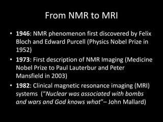
![Bloch Equation – Gradient Fields
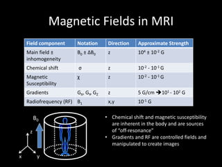
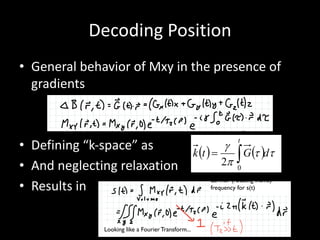
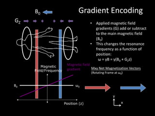
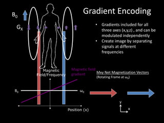
• Gradient coils create changes in the magnetic field versus
position
• Changes precession frequency to be a function of position
(enabling image formation):
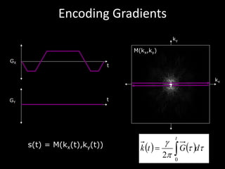
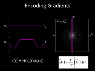
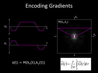
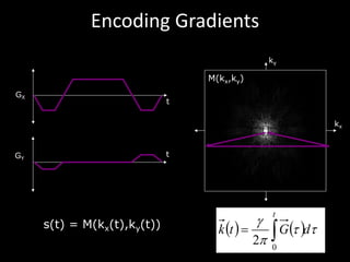
G(t) = [GX (t), GY (t), GZ(t)]
~B(~r, t) =
2
4
0
0
B0 + ~G(t) · ~r
3
5
!0 = (B0 + ~G(t) · ~r)
d ~M(t)
dt
= ~M(t) ⇥ ~B(t) +
2
4
1/T2 0 0
0 1/T2 0
0 0 1/T1
3
5 ~M(t) +
2
4
0
0
M0/T1
3
5](https://image.slidesharecdn.com/principlesofnmrimaging-pederlarsonenc2017-200204185843/85/Principles-of-N-MR-Imaging-9-320.jpg)