Essay Writing Service http://StudyHub.vip/Annotating-Soundscapes

1. Annotating Soundscapes
Dirkjan Krijnders1
Maria E. Niessen2
Tjeerd C. Andringa3
Auditory Cognition Group
Department of Artificial Intelligence
University of Groningen
P. O. Box 407
9700 AK Groningen
The Netherlands
ABSTRACT
We describe a soundscape annotation tool for unconstrained environmental sounds. The tool
segments the time-frequency-plane into regions that are likely to stem from a single source. A
human annotator can classify these regions. The system learns to suggest possible annotations
and presents these for acceptance. Accepted or corrected annotations will be used to improve the
classification further. Automatic annotations with a very high probability of being correct might
be accepted by default. This speeds up the annotation process and makes it possible to annotate
complex soundscapes both quickly and in considerable detail. We performed a pilot on
recordings of uncontrolled soundscapes at locations in Assen (NL) made in the early spring of
2009. Initial results show that the system is able to propose the correct class in 75% of the cases.
1. INTRODUCTION
Humans can recognize events in the sonic environment (soundscape) seemingly effortlessly.
However, this ability thus far eludes our technical abilities1. Automatic sound recognition has
important applications in fields as diverse as environmental noise monitoring, robotics, security
systems, content-based indexing of multi-media files, and even modern human-system
interfaces. Most sound recognition research is aimed at improving one aspect of these application
domains, such as speech recognition or music genre detection. These limited domain solutions
can rely on domain dependent assumptions that simplify the problem considerably. For example,
within music classification2 or speech recognition3 it is typically assumed that the input does not
1 j.d.krijnders@ai.rug.nl, 2 m.niessen@ai.rug.nl, 3t.andringa@ai.rug.nl

2. contain multiple uncorrelated streams of sonic evidence. As a consequence, stream segregation
and other problems are defined out of the problem-space and are not addressed scientifically.
In contrast to domain specific solutions, a general sound recognition system should be robust to
the complexities of unconstraint soundscapes, such as strong and varying transmission effects
and concurrent sources. To handle real-world complexities, human perception relies on signal-
driven processing, but also on contextual knowledge and reasoning4. Therefore, a general sound
recognition system should comprise an interaction of signal-driven techniques and interpretation
of the context.
This paper focuses on the development of a tool to facilitate real-world sound annotation for
training and benchmark purposes. It uses a set of simple algorithms to detect sonic events and to
classify these events. The interaction between semantic content, in the form of annotations, and
signal-based evidence forms the basis of future, more general, sound recognition systems.
The annotation of everyday sounds must lead to an adequate description of the content of a
sound-file in terms of the interval in which an event occurred. Annotation is a time-consuming,
and knowledge intensive task, which is usually quite boring as well. This is probably the reason
why there is currently only a single annotated database of sounds in realistic everyday
conditions5. Carefully selected everyday sounds in benign conditions have been used in other
studies6,7. However for these sounds the annotation problem is trivialized, because the data sets
contain single sound events in a single file.
There are many difficulties associated with real-world sound annotation:
• The great within class diversity of sounds (e.g. cars at different distances and speeds) in
combination with the co-occurrence of other classes makes it difficult to interpret a visual
rendering of the signal as spectrogram and to annotate the visual representation without
listening to the sounds in context. Visual inspection of spectro-temporal representations is an
important aid for annotation, but attentive listening to the sound is essential.
• Sonic events are often difficult to recognize using sound as the only modality. It is important
to annotate the sound during, or soon after, recording. The use of video information can be
very helpful whenever the sound sources are clearly visible and easily attributable (which is
often not the case).
• Anecdotic evidence suggests that annotation by someone who was not present when the
sound was recorded is much more error-prone and often many sounds cannot be annotated in
detail. For example, the difference between cars, truck, busses, and even motorcycles is
usually not at all obvious.
• The co-occurrence of multiple qualitatively different sonic events and sound producing
processes can lead to very complex signals, e.g. coffee-making in a lively kitchen. In these
cases it is difficult to track multiple uncorrelated processes and describe each in detail. One
might aim to annotate the so-called foreground or, alternatively, the events that attract
attention. However, this creates the new problem of determining what attracts attention or
what to assign to the foreground.
• The large number of individually distinguishable events of a similar kind, such as singing
birds in a forest, entails a lot of repetitive work.

3. • Realistic environments contain many barely audible events, e.g. distant speakers, which
might or might not be included in the annotation. Not including these might unjustly punish a
detection system that detects the valid, but unannotated, events. Conversely, including even
the faintest events is both time-consuming and prone to classification errors.
• Finally, the determination of the precise moment of the start and end of audible events is
subject to similar difficulties as those in the previous point. Especially the detection of the
on- or offset of a gradually developing event, like a passing car in a complex environment, is
often quite arbitrary. If the measure of success of a recognition system is based on
determining the intervals in which events occur, the system is punished for any deviation of
this arbitrary choice.
The difference between annotators who were present and who were not, suggests that the sonic
evidence may often be insufficient (for the human listener). This poses a fundamental problem
for each sound-only annotation or recognition system, whether human or machine; a correct
recognition result may simply be impossible. Hence, a perfect ground-truth is not a realistic goal
for a real-world sound recognition system. Instead, a performance equivalent to human
performance when not present during recording is more appropriate.
The current paper focuses on an annotation tool that helps to provide more insight in these
problems and helps to alleviate a number of them. It assists a human annotator by reducing the
number of repetitive actions by automatically suggesting annotations based on previous
annotations. This allows for the human annotator to accept the suggested annotation simply as an
instance of the proposed class, instead of having to select it from a (long) list of possible classes.
Within the annotation system we try to maximize the probability that the true event class is on
top of the list. Initially this list is simply alphabetic. During manual annotation the class list is
reordered according to the estimated probability that a certain event is an instance of the most
likely classes.
In the next section, we will give an overview of the annotation system. Furthermore, we present
the data on which it is tested. In the third section we will give the results of a pilot-experiment on
a set of real-world recordings. The paper ends with a short discussion of the annotation process.
2. METHODS
In this section we first describe the data set that is used to test the annotation system. This system
is based on processing sound in the spectro-temporal domain. Therefore, the sound signal is first
pre-processed, which will be explained in part B. Subsequently, we describe how the sound is
segmented into regions that are likely to include the most energetic spectro-temporal evidence of
the main sources. In part D we show how these regions are described in terms of a feature vector,
and how this feature vector is used to classify the regions. The section is concluded with a
system overview, which is shown in Figure 1.
A. Dataset
The dataset was collected under different weather conditions on a number of days in March 2009
in the town of Assen (65,000 inhabitants, in the north of the Netherlands). The recordings were
made by six groups of three students as part of a master course on sound recognition. Each group
made recordings of three minutes at six different locations: a railway station platform, a
pedestrian crossing with traffic lights, a small park-like square, a pedestrian shopping area, the

4. edge of a forest near a cemetery, and a walk between two of the positions. Recordings were made
using M-Audio Microtrack-II recorders with the supplied stereo microphone at 48 kHz and 24
bits stereo. This data, with annotations by the students, will be made available on http://
daresounds.org.
B. Preprocessing
Conversion to the time-frequency domain is performed by a gamma-chirp filter-bank8 with 100
channels. The filters are given by:
hgc = a tN-1 e-2 π b B(fc)t ej(2πfc t + c log(t))
with N = 4, a = 1, b = 0.71 and c = -3.7. fc is the channel center frequency. The center
frequencies are equidistant on a logarithmic axis between 67 Hz and 4000 Hz. The channel
bandwidth B(fc) is given by:
B(fc) = 24.7 + 0.108 fc
The output of the filter is squared and leaky-integrated with a channel-dependent time-constant:
τc = max(5, 2/fc) ms. The resulting time-energy representation is down-sampled to 200 Hz and
converted to the decibel domain. The resulting matrix of 100 channels with time-energy values is
termed ‘cochleogram’.
Sound data
Section 2.A
Cocleogram
Section 2.B
Segmentation
Section 2.C
Segments
with feature vectors
Section 2.D
Manual
Annotation
Section 2.F
Update kNN data
Section 2.E
update
distribution on non-
annotated segments
Section 2.F
Accept
Automatic
Annotation
Section 2.F
Remove
unannotated/unaccepted
segments
Section 2.F
Automatic
annotation
Section 2.F
Annotations with
spectral temporal
extend
Figure 1. Overview of the assisted annotation system. The two gray blocks are the only places of human
intervention.

5. This cochleogram representation shows minimal biases towards certain frequencies or points in
time. For example, unlike an FFT-based representation a cochleogram does not show frequency
dependent spectral leakage, which occur due to windowing effects when excited by a sine-sweep.
This entails that visible details reflect signal properties and not processing artifacts. A
cochleogram shows a combination of sinusoidal/tonal (horizontal), pulse-like (vertical), and
noisy components, depending on the sound signal. While channel-dependent shapes characterize
pulses and tones, noise is characterized by channel-dependent energy fluctuations that are
normally distributed.
Many sources produce predominantly sinusoidal (harmonic) or pulse-like sounds (impact
sounds)7. Thus measuring the local strength of tonal and pulse-like cochleogram contributions is
informative of source identity and may be used in a feature vector. The local tonal and pulse-like
contributions correlate to the height of the local energy value compared to neighboring values.
These are called the peaks-above-surrounding (PAS) values9,10 and can be computed for both
sinusoidal (PAS_S) and pulse-like (PAS_P) contributions. Both measures are expressed in terms
of the standard deviation of noise. Strongly positive or negative values (e.g. more that three
standard deviations from the mean of the noise) indicate values that are unlikely to originate
from noisy (broadband) components.
Local PAS values are calculated through channel dependent filtering of the cochleogram (see
figure 2). The filter for tones is designed by measuring the width of the energy-peak of a pure
tone (in the frequency direction). This width is asymmetric, which is taken into account. The
width is measured at an energy value corresponding to two standard deviations of white noise
Frequency
(Hz)
time [s]
0.5 1
1340
460
160
48
500 1000
0
10
20
30
40
50
60
70
Frequency [Hz]
Energy
[dB]
400 450 500
40
45
50
55
60
!nths
sb1 sb2
Frequency [Hz]
Energy
[dB]
Frequency
(Hz)
time [s]
0.5 1
1340
460
160
48
500 1000
0
10
20
30
40
50
60
70
Frequency [Hz]
Energy
[dB]
400 450 500
40
45
50
55
60
PAS !n
Frequency [Hz]
Energy
[dB]
sb1
sb2
Figure 2. The left panels show two cochleograms of pure tones, in clean situations (upper) and in 0 dB white noise
(lower). The middle and right panels show the energy profile at t=0.5 s. The upper panel show the derivation of the
filter width (sb1 and sb2) at ths times the standard deviation σn of white noise below the energy maximum. The
lower panel shows the application of the filter in noisy conditions. The difference between the mean energy at sb1
and sb2, and the energy at the TF point is the PAS_S.

6. under the energy maximum. Filtering corresponds to averaging the energy at the filter-width on
both sides of the time-frequency point and subtracting the average from the energy value at the
center. This value is normalized with the local standard deviation of white noise to yield the local
PAS_S value. The computation of the pulse-like local contribution, PAS_P, is identical, except
that the local width of a perfect pulse (in the temporal domain) is used.
C. Segmentation
The segmentation strategy is fairly basic. It is aimed at the inclusion of spectro-temporal maxima
in the form of blobs in the spectral and/or temporal direction. These blobs become prominent by
subtracting a strongly smoothed cochleogram from the original. The cochleogram is smoothed in
the temporal direction through leaky integration with a time-constant τ = 5 s. The time constant τ
determines the separation between fast, typically foreground, sonic events and slow, typically
background, events. The leaky integration operation corresponds to a delay in the expression of
mean energy values that is corrected by time-shifting the resulting values backwards with the
time-constant. This time-shift leads to a delay equal to the time-constant, which is not
problematic for off-line processing, but that is not desirable for online and real-time processing.
The temporal smoothing of time-series x(t) to yield xs(t) is defined by:
xs(t) = x(t-Δt) e(-Δt /τ) + x(t) (1-e(-t/τ))
Δ denotes the frame step of 5 ms. In addition to temporal smoothing, the cochleogram is also
smoothed in the frequency direction by taking a moving average over 7 channels. The difference
between the original cochleogram and the smoothed cochleogram can be termed a fast-to-slow-
ratio and is expressed in dB.
The regions with a fast-to-slow-ratio of more than 2 dB are assigned a unit value in a binary
mask. This mask is smoothed with a moving average in both the temporal direction (25 ms) and
the spectral direction (5 channels). The final mask is obtained by selecting average mask values
greater than 0.5, which smoothens region perimeters and reduces the number of supra-threshold
time-frequency points in the inner-regions of the mask that lead to small holes in the mask. The
final segmentation step is the estimation of individual coherent regions in the mask and to assign
a unique number to each region. The smallest bounding box that contains the whole region is
used to represent the region graphically (see figure 3). There are no special safeguards to ensure
either that each region represents information of a single source, or that all information of the
source is included in the regions. For example, when two cars pass at approximately the same
time, a single region will represent both. Alternatively, sounds that are partially masked by
(slowly developing) background sounds tend to break up into a number of smaller regions, that
are each less characteristic of the source. Nevertheless, the current settings seem able to include
important source information of a wide range of sources.
D. Feature vectors
The feature vectors must describe the source information represented by the regions. The 37-
dimensional feature vector represents properties related to the physics of the source. Note that
normal approaches to environmental sound feature estimation11 make no effort to include source
physics other than representing frequency content. The use of the PAS-values allows us to

7. attribute signal energy to tonal, pulse-like, or noisy contributions, which result from either source
limitations or transmission effects. Table 1 describes the feature vector.
The feature vector reflects the channel contributions per region, the fast-to-slow ratio, and the
distribution of tonal (PAS_S) and pulse-like (PAS_P) contributions. These signal descriptors are
represented by 7 different percentile values from the histogram of the local indicators. Different
percentile values might be indicative for different classes. For example, the 90 and 95 percentile
values might be highly indicative for footsteps in noise, while the other percentiles might not
discriminate from a the noisy contribution in a car passage.
Table 1: Region feature vector description
Feature Dim Percentile or range Description
Size 1 > 0.02 Fraction of spectro-temporal area equivalent to 1 s
Channel mean 1 1 - 100
Average channel number (1 is highest, 100 is lowest). This
corresponds to average log-frequency contribution.
Channel std 1 < 50 Provides a single number indication of the channel spread.
Fast-to-Slow-Ratio 7 [ 5 10 25 50 75 90 95 ]
The distribution of Fast-to-Slow-percentiles provides information
about the distribution of strong foreground values
PAS_S 7 [ 5 10 25 50 75 90 95 ]
The distribution of PAS_S values provides information about the
distribution of strong sinusoidal contributions.
PAS_P 7 [ 5 10 25 50 75 90 95 ]
The distribution of PAS_P values provides information about the
distribution of strong pulse-like contributions.
Channel distribution 7 [ 5 10 25 50 75 90 95 ]
The channel distribution provides more detailed information about
the pattern of contributing channels.
Channel spread 3 5-95, 10-90, 25-75
Provides more detailed information about the channel spread as
the difference in channel numbers between three percentile pairs
of the channel distribution
Frame spread 3 5-95, 10-90, 25-75
Provides more detailed information about the temporal spread as
the difference in frame numbers between three percentile pairs of
the frame distribution
E. Classification
Classification of regions based on the feature vector must lead to proposed classes for regions
similar to annotated regions. The classifier should function in an on-line fashion and must not
require long re-training phases. Additionally, the classifier should be able to function with
minimal training data. This combination of demands suggests a simple k-nearest-neighbor (kNN)
classifier12. Such a classifier stores all training feature vectors in a matrix. It classifies each
region by calculating the Euclidian distance d to all vectors in the training matrix and selecting
the k closest training examples which each represent an example of a single class. A simple
majority voting system is used to determine the best class for the region. To create a distribution
over multiple classes we count the number of occurrences a class in the top k = 5 and divide this
by (k * d / Σ d) to get a number indicating the match.
F. System overview
An overview of the annotation system is given in Figure 1. The system loads, pre-processes, and
segments the data of a single file and presents the result to the user. First, the user selects a
region. The selected region can be played as sound and a matching class can either be selected
from a class-list or added to the class-list. Initially the list is ordered alphabetically, but when
sufficiently matching examples of the class have been encountered, the top-positions on the list
will be ordered according to class-likelihood. After class assignment, the kNN training matrix is

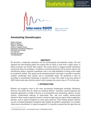
8. extended with the feature vector of the region. If the match of a class exceeds a threshold (here
set to p>0.04), it is automatically classified as that class. If the match exceeds 0.01, the region
will be conditionally classified, which entails that the user has to accept the classification before
it is included in the kNN training matrix. Regions that end up without annotation are discarded
after the user decides that the file is annotated in sufficient detail.
To measure the performance of the system we track the class-rank of manually annotated
regions, the number of automatically annotated regions, and the number of accepted regions. The
number of discarded regions is a measure for the performance of the segmentation. The final
output of the system is a list of classes assigned to regions.
3. RESULTS AND DISCUSSION
Measuring the performance of the system in meaningful numbers is difficult. A sensible measure
is the time saved by this system compared to full manual annotation of start and stop times of the
sound events. However each annotation session will result in different annotations due to the
reasons formulated in the introduction. This makes a fair comparison difficult. Furthermore the
current system is not yet sufficiently user-friendly to allow a good comparison. Alternatively we
measured how often the correct class was suggested by the kNN classifier. The results are shown
in table 2. When a class is either not annotated yet or misclassified, it is marked as
“alphabetical”, otherwise it is ranked as first or second. Without automated annotations one
expects an average rank equal to half the number of classes. Note that with k = 5 it is possible to
have 5 different classes in the list, but third, fourth or fifth ranked classes did not occur in the
test.
The current system is a first installment of the annotation tool. Its initial performance is
encouraging, but each aspect can and must be improved before it is truly useful. The further
Frequency
(Hz)
time [s]
115 120 125 130 135 140
2480
1640
1080
710
460
300
200
130
80
Car
Auto.
Bird
Auto.
Bird
Manual
MotorBike
Manual
Unknowns
Unknowns
Figure 3. The cochleogram of several passing cars. Darker means more energy. Solid lines denote manual
annotation. Dashed lines denote automatic classification, the dash-dotted lines denote still unclassified regions.
The cars are segmented in the pink boxes. A bird is segmented in the green box. The purple boxes are not (yet)
annotated.

9. improvement of the tool will depend strongly on an improved understanding of the annotation
process, which in turn is a special form of listening. Initial experience with assisted annotation
indicates that the annotator does not analyze the file from start to end, but instead prefers to focus
either on individual environmental processes or on individual auditory streams. This allows
maximal benefit from process/stream dependent knowledge. It is possible that everyday
listening13 reflects this so that at most one stream is analyzed with all available knowledge: the
focus of auditory attention. All other streams are analyzed in less detail. This observation in
combination with and the annotation problems formulated in this paper suggest that the question
“What do we do when we listen” should become a focus of active research.
ACKNOWLEDGMENTS
J.D. Krijnders' work is supported by The Netherlands Organization for Scientific Research under
Grant 634.000.432 within the ToKeN2000 program. M.E. Niessen's work is supported by
SenterNovem (Dutch Companion project grant no. IS053013). This research is also supported by
Foundation INCAS3, Assen, The Netherlands.
REFERENCES
1 Cano, P. “Content-based audio search: from fingerprinting to semantic audio retrieval”. Ph.D. Thesis. Pompeu
Fabra University (2006)
2 Jean-Julien Aucouturier, Boris Defréville, and Francois Pachet. “The bag-of-frames approach to audio pattern
recognition: A sufficient model for urban soundscapes.” J Acoust Soc Am, 122, 881-891 (2007).
3 Douglas O'Shaughnessy. “Automatic speech recognition: History, methods and challenges.” Pattern Recognition,
41, 2965-2979 (2008).
4 Maria E. Niessen, Leendert van Maanen, and Tjeerd C. Andringa. “Disambiguating sound through context.”
International Journal on Semantic Computing, 2(3), 327-341 (2008).
5 M.W.W. van Grootel, T.C. Andringa (2009) and J.D. Krijnders. “DARES-G1: Database of Annotated Real-world
Everyday Sounds.” DAGA-NAG 2009, Rotterdam
6 Marcell, M. E., Borella, D., Greene, M., Kerr, E., and Rogers, S. “Confrontation naming of environmental sounds.”
Journal of Clinical and Experimental Neuropsychology, 22, 830-864 (2000).
7 Gygi, B.; Kidd, G. R. & Watson, C. S. “Similarity and categorization of environmental sounds.” Perception &
Psychophysics, 69, 839-855 (2007).
8
Toshio Irino and Roy Patterson. “A time-domain, level-dependent auditory filter: The gammachirp”. J. Acoust. Soc.
Am. 101(1), 412-419 (1997).
9 Johannes D. Krijnders, Maria E. Niessen and Tjeerd C. Andringa, “Sound event identification through expectancy-
based evaluation of signal-driven hypotheses,” Pattern Recognition Letters, accepted, (2010)
10 Johannes D. Krijnders and Tjeerd C. Andringa, “Tone, pulse, and chirp decomposition for environmental sound
analysis,” Audio, Speech and Language Processing, IEEE Transactions on, submitted, (2010)
11 Cowling, M. and Sitte, R. “Comparison of techniques for environmental sound recognition.” Pattern Recognition
Letters, 24(15), 2895-1907 (2003)
12
Richard O. Duda, Peter E. Hart and David G. Stork, Pattern Classification, 2nd Edition (Wiley-Interscience, New
York, 2000)
13 Gaver, W. W. What in the World Do We Hear?: An Ecological Approach to Auditory Event Perception. Ecological
Psychology (1993)
Table 2: Results of an annotation session on the Assen dataset (N = 101)
alphabetical first second total
15% 74% 13% 100%