1. Physically Informed Subtraction of a
String’s Resonances from Monophonic,
Discretely Attacked Tones :
a Phase Vocoder Approach
by
Matthieu Hodgkinson
A thesis presented in fulfilment of the requirements for the Degree of
Doctor of Philosophy
Supervisor: Dr. Joseph Timoney
Department of Computer Science
Faculty of Science and Engineering
National University of Ireland, Maynooth
Maynooth, Co.Kildare, Ireland
May, 2012
2. “I do not define time, space, place, and motion, as being well known to all.”
Isaac Newton
I
3. Declaration
This thesis has not been submitted in whole or in part to this
or any other university for any other degree and is, except
where otherwise stated, the original work of the author.
Signed:
Matthieu Hodgkinson
II
4. Abstract
A method for the subtraction of a string’s oscillations from monophonic,
plucked- or hit-string tones is presented. The remainder of the subtrac-
tion is the response of the instrument’s body to the excitation, and poten-
tially other sources, such as faint vibrations of other strings, background
noises or recording artifacts. In some respects, this method is similar to a
stochastic-deterministic decomposition based on Sinusoidal Modeling Syn-
thesis [MQ86, IS87]. However, our method targets string partials expressly,
according to a physical model of the string’s vibrations described in this the-
sis. Also, the method sits on a Phase Vocoder scheme. This approach has
the essential advantage that the subtraction of the partials can take place
“instantly”, on a frame-by-frame basis, avoiding the necessity of tracking the
partials and therefore availing of the possibility of a real-time implementa-
tion. The subtraction takes place in the frequency domain, and a method
is presented whereby the computational cost of this process can be reduced
through the reduction of a partial’s frequency-domain data to its main lobe.
In each frame of the Phase Vocoder, the string is encoded as a set of par-
tials, completely described by four constants of frequency, phase, magnitude
and exponential decay. These parameters are obtained with a novel method,
the Complex Exponential Phase Magnitude Evolution (CSPME), which is
a generalisation of the CSPE [SG06] to signals with exponential envelopes
and which surpasses the finite resolution of the Discrete Fourier Transform.
The encoding obtained is an intuitive representation of the string, suitable
to musical processing.
III
5. Acknowledgments
Tout d’abord, je voudrais exprimer une reconnaissance profonde envers ma
m`ere et mon p`ere, qui n’ont jamais cess´e de me montrer et de me donner leur
support. Mais je voudrais aussi adresser une note particuli`ere `a Andr´e, qui
en quelque sorte a tenu pour moi, sans que je m’en rende compte d’abord,
un rˆole de m´ec`ene au cours de mes ann´ees d’universit´e. J’en profite aussi
pour rendre hommage `a un grand ami, Nicolas Perrin, qui nous a quitt´e
Novembre dernier, et qui, j’en suis sˆur, aurait ´et´e tr`es fier de dire que, ¸ca
y’est, Hodgkinson, il est docteur. Et moi Nico, j’aurais ´et´e fier de pouvoir te
rendre fier comme ¸ca.
Back in Ireland, I would like to thank my supervisor Dr. Joseph Timoney,
for the guidance he gave me throughout my PhD. And beyond my supervisor,
there is the entire department of Computer Science of NUI Maynooth, with
its Head, lecturers, technicians and secretaries, who have all been admirably
helpful. I guess you get this nowhere like in Ireland.
IV
6. Foreword
The sensation of sound occurs when our tympanic membrane is set in a
vibrational motion of appropriate amplitude and frequency. The vibration
of our tympanic membrane is normally the effect of an analogue oscillation
in the ambient air pressure, and thereby it can be said that the medium of
sound is air. However, sound can also be experienced underwater, so water
can also be the medium of sound. In fact, even solids transmit sound: shake
a light bulb beside your ear, and even though it is hermetically enclosed in
glass, you will hear the filament shaking.
Sound has a number of media. In the 20th
century, the domestication of
electricity as a medium for sound has revolutionised our experience of music.
Now sound can be stored, processed, and even generated. Electronic ma-
chines with keyboard interfaces use mathematical algorithms to create tones
previously unheard. In the second half of the past century, these synthesiz-
ers become so popular as to grow in a family of instruments of their own.
Most notably, the success of the Moog synthesizer, commercialised first in
the 1960s [PT04], is monumental. The Doors, the Beatles, Pink Floyd, to
name just a few, are all names this instrument contributed to the success of.
Technically speaking, the Moog uses a paradigm for the synthesis of mu-
sical signals called subtractive synthesis, whose elementary principle is to
generate a harmonic or near-harmonic waveform of rich spectral properties,
and filter it thereafter in inventive manners. Other paradigms used in the
60s, 70s and later include additive synthesis and FM (Frequency Modulation)
synthesis [Cho73]. During this time, computers become more powerful and
V
7. affordable, and digital sound synthesis emerges. A remarkable development
of that time in sound synthesis is the birth of physical modeling, which aims
at emulating in a computer the physical mechanisms that lead to the produc-
tion of sound waves. Hiller and Ruiz take a Finite Difference (FD) approach
to approximate the solutions to the Partial Differential Equations (PDEs)
derived from the physical analysis of vibrating bodies [HR71a, HR71b]. In
the early 80s, Karplus and Strong introduce a digital system which, with
a simple delay line and averaging filter arranged in a feedback loop, pro-
duce tones whose resemblance with string tones is uncanny. The method
inspires Julius Smith to develop the theory of Digital Waveguide Synthesis
[III92], which models d’Alembert’s (1717-1783) solution to the wave equation
in delay lines, connected in a digital loop enriched with various types of fil-
ters to emulate the various phenomena undergone by the waves during their
propagation: frequency-dependent dissipation of energy, dispersion, and so
on.
The developments of this already successful sound synthesis paradigm
did nevertheless not stop here. In string tones, the instrument’s body was
problematic in the sense that it could not practically be modeled as a 3-
dimensional waveguide, meanwhile contributing – in some cases significantly
– to the timbre of the instrument. This problem was worked around with
the advent of Commuted Waveguide Synthesis (CWGS), which stores the
response of the body in a wavetable, and uses it as the input to the digi-
tal waveguide [KVJ93, Smi93]. The method shows a potential to producing
virtual instrumental parts hardly distinguishable from acoustic recordings,
VI
8. and this, in real time. Examples of the method can be found at the Web ad-
dress http://www.acoustics.hut.fi/~vpv/ (latest access: September 10th
,
2011).
Commuted Waveguide Synthesis requires the indirect response of the in-
strument’s body to the excitation of the string. This response is obtained
through a preliminary process commonly known as excitation extraction. A
string instrument’s note is recorded, and all sinusoidal components that are
not part of the body’s response are canceled. The residual is a burst of
energy, very short in some cases, slightly longer when the body shows rever-
berant qualities, but rarely exceeding a second. In the cases where the string
is materially flexible enough to show negligible inharmonicity, when the har-
monics are not too numerous and when the body does not show prominent
resonances, using the inverse of a string model [KVJ93] or a simple Sinusoidal
Modeling approach [MQ86, IS87] can yield satisfying results. However, when
some or none of these conditions are met, an unwanted residual of the string’s
resonances threatens to remain. Moreover, the interpolative nature of Sinu-
soidal Modeling Synthesis prevents the real-time processing of the input.
The intent of this thesis was initially to devise an automated method for
excitation extraction. A Phase-Vocoder approach proved convenient, and in
addition brought the possibility of a real-time implementation within reach.
This possibility raised the question “What could real-time add to excitation
extraction?”. Live musical effects was the answer. But live conditions are
different to the studio conditions where tones suitable for subsequent use in
digital waveguides should be recorded. Thereout emerged the paradigm of
VII
10. Publications
The following is an ordered list of the publications of the author:
1. Matthieu Hodgkinson, Jian Wang, Joseph Timoney, and Victor Laz-
zarini “Handling Inharmonic Series with Median-Adjustive Trajecto-
ries”, Proceedings of the 12th International Conference on Digital Au-
dio Effects (DAFx-09), Como, Italy, 2009.
2. Matthieu Hodgkinson, Joseph Timoney, and Victor Lazzarini “A
Model of Partial Tracks for Tension-Modulated, Steel-String Guitar
Tones”, Proceedings of the 13th International Conference on Digital
Audio Effects (DAFx-10), Graz, Austria, 2010.
3. Matthieu Hodgkinson “Exponential-Plus-Constant Fitting based on
Fourier Analysis”, JIM2011 – 17`emes
Journ´ees d’Informatique Musicale,
Saint-´Etienne, France, 2011.
IX
16. List of Figures
1 Isolating a note from a melody with unit-step windowing. . . . 7
1.1 Vertical forces onto string segment . . . . . . . . . . . . . . . 16
1.2 Simple model for pluck excitation . . . . . . . . . . . . . . . . 23
1.3 Coefficient series Ak for various plucking positions up . . . . . 26
1.4 Simple model for hit excitation . . . . . . . . . . . . . . . . . 28
1.5 Harmonic-index-dependent decay rate (upper plot) and fre-
quency deviation (lower plot) in semitones due to damping on
a Spanish guitar open E4 . . . . . . . . . . . . . . . . . . . . . 36
1.6 Harmonic-index-dependent decay rate (upper plot) and fre-
quency deviation (lower plot) in semitones due to damping on
an acoustic guitar open E4 . . . . . . . . . . . . . . . . . . . . 37
XV
17. 1.7 Frequency deviation in semitones due to stiffness on Span-
ish and acoustic guitar tones. The deviation of the partials,
clearly measurable and visible, is well approximated with the
inharmonic-series expression (1.33) (solid curve). Note : the
musical interval in semitones between two frequencies f2 and
f1 is calculated as 12 log2 f1/f2, hence the 12 log2 terms in the
legend. . . . . . . . . . . . . . . . . . . . . . . . . . . . . . . . 39
1.8 Fundamental Frequency & Inharmonicity Coefficient measure-
ments in an Ovation acoustic guitar open bass string. . . . . . 49
1.9 FF and IC models (dashed lines) fitted in previously presented
measurements (circles), using the Fourier-based method. . . . 55
1.10 Model of partial tracks based on time-varying (solid lines) and
fixed (dashed lines) Inharmonicity Coefficient, on top of the
Ovation E2 spectrogram. The focus is here on partials 53 to 55. 56
1.11 Presence of longitudinal partials in Spanish (top) and acoustic
(bottom) guitar spectra. Both are open bass E tones. . . . . . 58
1.12 Transverse series and transverse-driven longitudinal series in
a Steinway E2 piano tone. Transverse-longitudinal conflicting
partials are marked with crossed circles. . . . . . . . . . . . . 64
2.1 Discrete spectra of single complex exponential, synchronised
(top) and out-of-sync (bottom) in the Fourier analysis period. 75
2.2 Multi-component spectra, with negligible (top) and prejudicial
(bottom) overlap. . . . . . . . . . . . . . . . . . . . . . . . . . 78
XVI
18. 2.3 Rectangular and Hann windows, in time (top) and frequency
(bottom) domains. . . . . . . . . . . . . . . . . . . . . . . . . 83
2.4 Magnitude spectra of first four continuous windows. . . . . . . 88
2.5 Trend in spectra of 1st
-, 2nd
- and 3rd
-order continuous (solid
lines) and minimal (dashed lines) windows. . . . . . . . . . . . 89
2.6 Acoustic guitar spectra derived with 2nd
-order continuous (top)
and minimal (bottom) windows. Notice the steady noise floor
in the lower plot. . . . . . . . . . . . . . . . . . . . . . . . . . 92
2.7 Constant-power-sum property of Cosine windows. In the up-
per plot, the minimal overlap required is short of one, the con-
dition of equation (2.21) that i > 0 not being respected. The
lower plot respects this condition: see how the sum suddenly
stabilises over the interval where PQ + i windows overlap.
The coefficients of the cosine window were chosen randomly,
to emphasize the phenomenon. . . . . . . . . . . . . . . . . . . 94
2.8 Kaiser-Bessel window and window spectrum (normalised), for
two different zero-crossing settings. . . . . . . . . . . . . . . . 99
2.9 Gaussian infinite (solid lines) and truncated (dashed lines)
window (linear scale) and spectrum (decibel scale). The frequency-
domain approximation by the dashed line is only satisfying
when the time-domain lobe is narrow in relation to the anal-
ysis interval. . . . . . . . . . . . . . . . . . . . . . . . . . . . . 101
XVII
19. 2.10 Confrontation of truncated gaussian window with the mini-
mum two- (upper plot) and three-terms (lower plot) cosine
windows. Cosine windows here show narrower main lobes. . . 103
2.11 Fourier transform (solid line) and DTFT (dashed line) of a
discrete-time signal. In continuous time, the discrete signal is
expressed as a sum of sinc functions, which induces the rect-
angular windowing seen in the frequency domain, responsible
for the absence of components beyond |fs/2|Hz. . . . . . . . . 109
2.12 Periodicity of the DFT for complex (upper plot) and real
(lower plot) signals. . . . . . . . . . . . . . . . . . . . . . . . . 112
2.13 N-length DFT (circles) and FFT (crosses) big-oh computa-
tional complexity. . . . . . . . . . . . . . . . . . . . . . . . . . 116
2.14 “Full-cancelation time”, tdB, over the note’s fundamental pe-
riod, T0, measured for each harmonic (“Har. num.” axis) of
a number of notes (“MIDI note” axis) and four instruments,
from top to bottom: electric guitar, grand piano, double bass
(plucked) and harpsichord. The rule for successful cancelation
of a partial with exponential envelope approximated with a
constant-amplitude sinusoid is that tdB/T0 > P + 1, P being
the order of the window used. The median values tdB/T0 for
each instrument, in black, are shown in Table 2.3. . . . . . . . 128
2.15 The four parameters of our short-time sinusoidal model: fre-
quency (ωr), growth rate (γ), initial phase (φ) and amplitude
(A). . . . . . . . . . . . . . . . . . . . . . . . . . . . . . . . . 134
XVIII
20. 2.16 Summary of our parametric estimation of first-order amplitude
and phase complex exponential. The notation XM
N denotes an
FFT of length M using a cosine window of length N. “p.d”
stands for “peak detection”. . . . . . . . . . . . . . . . . . . . 143
3.1 Zero-padded signal (upper plot) and its autocorrelation (lower
plot). In the upper plot, the periodicity of the waveform is
highlighted with the time-shift, in dashed line, of the original
waveform by one period. This time shift corresponds to the
autocorrelation peak at index NFF. . . . . . . . . . . . . . . . 151
3.2 Peak index refinement with quadratic fit . . . . . . . . . . . . 153
3.3 Phase-Vocoder process: from the signal at its original time
indices, to the frequency domain, and back. . . . . . . . . . . 155
3.4 Granulation process: the original signal is first zero-padded
(top plot) before being granulated (lower plots, c.f. Equa-
tion (3.3)), time-aligned to zero (Equation (3.4)) and DFT-
analysed (Equation (3.5)). . . . . . . . . . . . . . . . . . . . . 159
3.5 Phase Vocoder setup for a finite-length input. A finite num-
ber of windows is necessary (here, 5) depending on the win-
dow length and overlap. Zero-padding the signal on either
end to accommodate windows outside the original interval is
a practical approach to the granulation process in computer
applications. . . . . . . . . . . . . . . . . . . . . . . . . . . . . 162
XIX
21. 3.6 Snapshot of the frequency-domain string cancelation process,
with the CSPME method introduced in Section 2.5.1 (top),
and with the CSPE method as originally introduced in [SG06]
(bottom). The partial index k of the peak standing at the
centre of the figure is 52. . . . . . . . . . . . . . . . . . . . . . 165
3.7 Spectrum before (dashed lines) and after (solid lines) cance-
lation, for minimal-sidelobe cosine window of order 2. Zero-
padding was used here for visual purposes, but is normally
unnecessary. . . . . . . . . . . . . . . . . . . . . . . . . . . . . 167
3.8 Time-domain segment before (top) and after (bottom) frequency-
domain cancelation of the main lobe. In the lower plot, the
dashed line is the time-domain segment after cancelation and
windowing. . . . . . . . . . . . . . . . . . . . . . . . . . . . . 168
3.9 Frequency-domain cancelation of overlapping partials. The
dominating peak (dotted line) is measured and canceled first.
Previously mere bulge, the dominated partial has now become
a peak (dashed line), and can be, in turn, measured and canceled.170
3.10 Unit-step-windowed string partial, modeling the attack of the
tone. . . . . . . . . . . . . . . . . . . . . . . . . . . . . . . . . 173
3.11 Unit-stepped hamming window. The dotted-line, standard
window exhibits the expected spectrum, with its minimal,
well-dented sidelobes. As the window goes unit-stepped, how-
ever (dashed line, solid line), it looses its optimal spectral
properties, with much higher sidelobes. . . . . . . . . . . . . . 177
XX
22. 3.12 Top: Acoustic guitar E2 (MIDI note 40). Bottom: Viola
(pizzicato) G5 (MIDI note 79). . . . . . . . . . . . . . . . . . . 178
3.13 Detecting the transverse partials in an inharmonic spectrum
with a local linear approximation. The frequencies of the cir-
cled peaks are used in a Linear Least Square fit. In the upper
plot, the series behaves as expected, nearly harmonically. In
the lower plot, however, an unexpected behaviour is visible,
rendering the linear approximation (dashed lines) unsuitable. . 188
3.14 Peaks, bulges and caves: three concepts necessary to decide
securely which of the two overlapping partials should be can-
celed first. Even when they are the effect of one same partial,
a curvature minimum (bulge) does not always coincide exactly
with a magnitude maximum (peak). . . . . . . . . . . . . . . . 193
4.1 Frequency-domain synthesized string spectrogram (top) and
spectrogram after time-domain re-synthesis (bottom). Due
to the overlap (here, 5) of the analysis frames, these are not
equal. Notice the smearing, both horizontal and vertical, of
the spectral energy. . . . . . . . . . . . . . . . . . . . . . . . . 203
4.2 Harpsichord A4 (MIDI note 69) before (lighter shade) and
after (darker shade) string extraction. . . . . . . . . . . . . . . 204
4.3 Harpsichord A4 (MIDI note 69) before (top) and after (bot-
tom) string extraction. . . . . . . . . . . . . . . . . . . . . . . 204
4.4 Viola G5 (MIDI note 79), played pizzicato. . . . . . . . . . . . 207
XXI
23. 4.5 Stratocaster D3 (MIDI note 50): example of noise which is
neither string nor excitation . . . . . . . . . . . . . . . . . . . 208
4.6 Martin E5 (MIDI note 76) after string extraction. The “events”
in the noise floor are movements of the performer during record-
ing, only audible after string extraction. . . . . . . . . . . . . 209
4.7 Acoustic guitar open D (MIDI note 50). In this example, the
sympathetic vibrations of the other open strings are clearly
audible in the processed sound. . . . . . . . . . . . . . . . . . 209
4.8 Double Bass A2 (MIDI note 45) before (lighter shade) and
after (darker shade) string extraction: a constant-amplitude
model, for this heavily damped tone, yields a result of equiv-
alent quality. . . . . . . . . . . . . . . . . . . . . . . . . . . . 212
4.9 Nylon-string acoustic guitar D3 (MIDI note 50) with CSPME
(top) and a contant-amplitude (bottom) models for cancelation.213
4.10 Acoustic Guitar E2 (MIDI note 40): Spectrum after sub-
traction (upper plot, solid line) should be lesser than before
(dashed line). CSPME measurement of leftmost circled peak
largely erroneous, responsible for added energy. In time-domain
output (lower plot), results in outstanding sinusoidal grain. . . 217
4.11 How cosine windows of higher order gather their energy closer
to their center. . . . . . . . . . . . . . . . . . . . . . . . . . . 219
4.12 For testing, the windowing was synchronised with the attack
sample, ν. The shape (triangular) an line style (solid and
dashed) of the windows are for visual purpose only. . . . . . . 220
XXII
24. 4.13 Acoustic Guitar E2 (MIDI note 40) with onset overlap 0/5
(top), 1/5 (middle) and 2/5 (bottom) . . . . . . . . . . . . . . 221
4.14 To avoid the discontinuity inherent to the unit-step modeling
of the attack, the output should be cross-faded with the input
over a few samples after ν. . . . . . . . . . . . . . . . . . . . . 223
4.15 Spanish guitar open bass E (MIDI note 40). Left column: both
transverse and phantom partials are sought and canceled; right
column: only transverse partials are canceled. Upper row: the
window length is set to the minimal length; lower row: the
window length is thrice the minimal length. The “burbling”
in the upper row is a confusion of our algorithm, caused by a
misleading situation of overlap. . . . . . . . . . . . . . . . . . 225
4.16 “Burbling”, caused by the slowly-incrementing phase differ-
ence in the sliding analysis of overlapping partials, of frequen-
cies ω1 and ω2. In subplots 1 and 5, the phase of the two
partials is equal at the centre of the analysis, and in 3 and 7,
is is opposite. . . . . . . . . . . . . . . . . . . . . . . . . . . . 226
4.17 Acoustic guitar E2 (MIDI note 40) string extraction spectro-
grams omitting (top) and accounting for (bottom) the phan-
tom partials. . . . . . . . . . . . . . . . . . . . . . . . . . . . . 229
4.18 Acoustic guitar E2 (MIDI note 40) string extraction waveform,
omitting (lighter shade) and accounting for (darker shade) the
phantom partials. . . . . . . . . . . . . . . . . . . . . . . . . . 229
XXIII
25. 4.19 Grand piano F#4 (MIDI note 54) string extraction spectro-
grams omitting (top) and accounting for (bottom) the phan-
tom partials. . . . . . . . . . . . . . . . . . . . . . . . . . . . . 230
4.20 Grand piano F#4 (MIDI note 54) string extraction waveform,
omitting (lighter shade) and accounting for (darker shade) the
phantom partials. . . . . . . . . . . . . . . . . . . . . . . . . . 230
XXIV
26. List of Tables
1.1 Measurements regarding the audibility of inharmonicity in
three instruments . . . . . . . . . . . . . . . . . . . . . . . . . 41
1.2 String model developed in this chapter. . . . . . . . . . . . . . 66
2.1 0th
, 1st
-, 2nd
- and 3rd
-order continuous and minimal windows. . 90
2.2 Recapitulated advantages and disadvantages of windows seen
in this thesis. . . . . . . . . . . . . . . . . . . . . . . . . . . . 107
2.3 Median values of the ratio tdB/T0 across all harmonics of all
notes, for four instruments of contrasting character. . . . . . . 129
2.4 The decay rate γω and magnitude ω∆ of the non-constant part
of the fundamental frequency of string tones can be used to
estimate the ratio tdB/T0. The measurements shown here are
from fortissimo tones of an Ovation acoustic guitar, spanning
two octaves and a major third. The evaluation of tdB/T0 indi-
cates here that, in the worst case, a second-order cosine win-
dow can be used in a cancelation process using a constant-
frequency model, and yet ensure an output wave of less than
-60dBFS. . . . . . . . . . . . . . . . . . . . . . . . . . . . . . . 132
XXV
28. Chapter 0
Introduction
This thesis proposes a novel method to extract the oscillatory components
issued from a string’s vibration in monophonic, plucked or hit string tones.
The method operates within a Phase Vocoder time-frequency representation
of the input tone, where a vertical process is repeated on a frame-by-frame
basis, independently of the state of previous or following frames. This pro-
cess consists of three steps: the detection and identification of the string’s
partials; the measurement in frequency, phase, magnitude and exponential
envelope of these partials; and their frequency-domain re-synthesis and sub-
traction. Upon completion, the tone is decomposed in a “string” part, that
consists of a set of partials that are completely determined by the above-
mentioned parameters, and the rest of the tone, which includes stochastic
elements and often sinusoidal elements as well, such as resonances of the
instrument’s body or faint vibrations of other strings. Conceptually, this
process is reminiscent of excitation extraction [LDS07], but here the term
1
29. string extraction is preferred, for reasons that are going to be developed in
the first section of this introductory chapter. Following this conceptual clar-
ification, we will delineate the range of tones that are suitable inputs to the
method, suggest applications of the method, and finally present the plan of
the main body of this thesis.
0.1 String extraction: conceptual definition
String extraction in a way can be regarded as some sort of sound source
separation, where there are two entities to separate, one simple, and one
complex. The simple entity is the “string” entity, and the complex entity
is “all the rest”. We cannot readily give a specific name to the latter, be-
cause itself may be decomposed into several sub-entities: the response of the
instrument’s body to the excitation, some vibrations of the other strings, a
recording noise floor, ambient noises, and so on. The reason why we nev-
ertheless group all these components into one entity is because our aim is
simply to extract the string, and it does not matter what this rest is – so
long as it is not so invasive that it compromises the working of our method,
which looks for a prominent time-frequency structure to the tone that it can
associate to a string model.
The signal processing paradigm closest to ours would presently be exci-
tation extraction. This paradigm was probably motivated by the advent of
Commuted Waveguide Synthesis (CWGS) [KVJ93, Smi93] in the early 90s,
although it is conceptually close to the decomposition of a signal into de-
terministic and stochastic parts, which stems back to the mid-80s [RPK86,
2
30. MQ86, IS87]. CWGS is a sound synthesis method for plucked or hit string
instruments where the string is modeled as a system of filters and the re-
sponse of the instrument’s body is used to excite the model. It is thereby
that the response of the body to the excitation is itself seen, in CWGS,
as an excitation. “Body response” and “excitation” may therefore be used
interchangeably.
To obtain this excitation, a standard deterministic-stochastic decompo-
sition may be used. However, there is a potential risk in this approach that
resonances of the body are mistaken for string partials, and mistakenly taken
away from the instrument’s body response. To avoid this, a model of the
string can be used as a guide to deciding whether a partial belongs with the
string or not. But then another risk arises, that sympathetic vibrations of
other strings are seen as part of the response of the body, which they are not
either.1
In our opinion, so long as a method cannot distinguish between body
resonances and sympathetic vibrations, an automatic method for excitation
extraction cannot be devised unless the assumption is made that the other
strings of the instrument are muted. Even then, stochastic energy that is not
part of the body response, such as the noise floor of the recording or acci-
dental ambient noises, might remain in the excitation. Another assumption
therefore has to be made is that the recording is of such quality that any
sound components that are part of neither the excitation nor the targeted
string are inaudible.
1
Unless muted, other strings are likely to respond indirectly to the excitation of the
target string and to vibrate sympathetically, because of the transmission of vibrations
through the bridge of the instrument.
3
31. Such optimal constraints can only be satisfied in carefully arranged studio
conditions. These constraints are relaxed in the context of string extraction,
extending the range of applications of the paradigm. But before the po-
tential applications are discussed, a moment should be spent to determine
what types of input are suitable to string extraction, both conceptually and
technically.
0.2 Suitable inputs
Before we begin discussing what inputs are suitable inputs, the distinction
should be made between inputs that are suitable at a conceptual level – from
which it makes sense to remove the vibrations of one or more strings – and
those suitable at a technical level – from which is is technically possible to
remove the vibrations of the string(s). An example of an input suitable at
both levels would be a pluck of a guitar string isolated in time. An example
of input suitable at a conceptual level, but not at a technical level, could be
a piano piece, because it is polyphonic, and our method currently does not
support polyphonic input. The distinction between conceptual and technical
suitability is thereby easy to make: a input, even if conceptually suitable, will
only be technically suitable if the technical means are built into the method
to deal with its complexity. What is the condition for conceptual suitability,
on the other hand, is not evident, and should be briefly discussed here.
The rumble of a train, one would probably agree, is not suitable to string
extraction. But what about a bowed violin melody? Separating the string
from the indirect response of the body to the bow and any other sort of
4
32. non-string sounds (such as the breathing of the violinist) makes sense, and
surely could have numerous applications. However, we are going to draw the
line around discretely attacked string tones. If this line were not drawn, then
it could be argued that sung tones are also suitable, and speech tones, and
so on, which would then make the string extraction paradigm a reduction
of source-filter modeling. In a way, it is, but as the reader will see by the
reading of Chapter 1, it is also an “augmentation” of source-filter modeling,
because string extraction relies on a string’s physical model, and the time-
frequency data collected during the process is given meaning through its
association to this model. A plucking position, for example, can be inferred
from the notches found in a string’s comb-like spectrum [TI01], or a gain
spectrum can be derived from the measurement of the decay rates of the
partials [KVJ93, VHKJ96], which may turn out to be typical of a Spanish
guitar or a plucked double bass. These are all timbre attributes that make the
specificity of discretely-attacked string tones, to the point that, even played
in isolation of the body response, the sinusoidal structure of a string still very
much sounds like a string. Conceptually suitable inputs are therefore inputs
whose time-frequency characteristics are inherent to the physical model that
will be described in Chapter 1: plucked or hit string tones, simply.
So ideally, we would present in this thesis a method that is flexible enough
to be able to deal with polyphonic parts of plucked string instruments. How-
ever, the intent was initially to devise an automated method for excitation
extraction for subsequent use in digital waveguides, and as such, was only
meant for monophonic tones – the conceptual generalisation to string ex-
5
33. traction only came at an advanced stage of the thesis’ genesis. As for all
sinusoidal analysis methods based on the FFT, the good resolution of the
partials is assumed in our method, and the difficulty of overlapping partials
may therefore require an entirely different approach, which is beyond the
scope of this thesis. Now the question must be asked as to what types of
inputs our method is technically capable of dealing with. Only after light
has been shed on this point can current applications can be discussed.
Chapter 4 tests the string extraction method described throughout this
thesis. All these tests were run upon monophonic string tones, each recording
featuring one note only. The time structure of the physical model developed
in this thesis is an approximation whereby the string’s vibrations are nil
until time t = 0, when they are instantly set into sinusoidal motion. In our
processing, this is viewed as a unit-step windowing of the sinusoidal motion of
the partials, which otherwise would have been vibrating ever since t = −∞.
The tone stops when all the vibrational energy is dissipated, when the string
is muted, or when the attack is renewed, either on a same note or a different
note. The muting of a note or its interruption by the plucking of an other note
can also be modeled by a product with a time-reversed unit-step function.
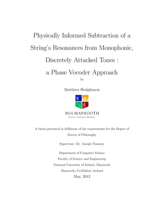
Our point here is that, even within a melodic phrase, a note can be taken
out of its context to reproduce the testing conditions of Chapter 4. The idea
is illustrated in Figure 1.2
Finally, some string instruments such as the piano, but also the dulcimer
2
In this figure, the unit-step windowing looks like rectangular windowing, but in our
processing mindset, we look at tones at the time scale of a STFT window, where it is
unlikely that the analysed tone is both attacked and muted. In this case, a unit-step
windowing expression seems more appropriate.
6
34. 0 1.1025 2.205 4.41
x 10
4
−1
0
1
Time (samples)
Amplitude
Melodic input
Unit−stepped input
Unit−step function
Figure 1: Isolating a note from a melody with unit-step windowing.
or the harpsichord feature courses of strings, arrangements of two or more
strings which vibrate together in the production of one same note. There
are several reasons for such facture, mainly a gain of loudness, but also an
increase of the “depth” of the sound, produced by strings that are very nearly,
but not exactly, tuned to unison. This is problematic for our method, which
has been devised in this thesis to deal with the pseudo-harmonic series of one
string only. In our collection of piano and harpsichord tones, the information
was not readily available whether tones were the contribution of a single
string or of courses of string. This consideration could therefore not be made
on a tone-by-tone basis, but it may account for some of the sense of pitch
that remained after string extraction in our least successful examples. With
regard to the extent of this thesis, we will consider that tones issued from
courses of strings are also eligible, only we will assume perfect unison tuning.
Without this assumption, a number of highly regarded instruments such as
the piano or the harpsichord would be excluded, while our method still gives
satisfying results for the greater part of their range.
7
35. 0.3 Applications of the present method for
string extraction
In summary of the previous section, the inputs suitable for our method
of string extraction are monophonic sequences of discretely-attacked string
tones. These sequences may reduce to one note only, or may be entire
melodies. Albeit restrained by the monophonic limitation, our method can
already be the starting point for a range of musical effects. In the view of
this type of application, the method has been developed as much as possible
to facilitate a real-time implementation. A Phase Vocoder approach – this
paradigm will be presented in detail in Chapter 3 – has therefore been pre-
ferred to a Sinusoidal Modeling Synthesis approach [MQ86, IS87], where a
real-time implementation is compromised by the fact that it uses interpola-
tion between measurement points to cancel the partials. This means that,
at frame a, it will have to wait for frame b – “much” later – to be processed
before interpolation and cancelation takes place. In our approach, the can-
celation takes place on a frame-by-frame basis. This does not reduce the
latency to zero, as the buffering of a few fundamental periods of the tone is
still required for the frequency-domain analysis and processing to take place,
but it reduces it substantially. How audible and inconvenient this minimal
latency is to the real-time effects made achievable by the method, and how
it can be worked around, is yet an open question.
The applications that gain from a real-time implementation are essen-
tially musical applications. The subtractive nature of our string extraction
8
36. method, as well as the underlying physical model and the original techniques
employed, render many “traditional” effects very accessible, and also bring
about original, physics-based effects. For example, a pitch-shifter/harmoniser
the likes of which is found in [LD99], but readily benefitting from the detec-
tion and cancelation of the partials of the string extraction process, seems
now fairly straightforward to implement, with the added guarantee that po-
tential sympathetic vibrations or body resonances, themselves, remain at
their original pitch. In combination with a pitch-shifter could come an “inhar-
monicity modifier”: the frequency of a string partial is not only determined
by the fundamental frequency, but also by the Inharmonicity Coefficient (IC).
A method original to this thesis, the Median-Adjustive Trajectories (MAT),
integrates the estimation of this coefficient in the peak detection. Upon string
extraction, the IC can be modified, virtually altering the physicality of the
string.
Another effect that the various innovations of this thesis may offer is a
real-time “sustain stretcher”. In contrast with a standard time stretcher,
a sustain stretcher would modify the decay rates of the partials without
slowing down or accelerating the frequency glide of the partials typical of
tension-modulated tones [HTL10]. This is achievable in real time thanks to
the CSPME, a generalisation of the CSPE [SG06] to exponential-amplitude
signals. This novel method returns the decay rate of partials on the basis of
a single frame, allowing for a modification “on the spot” of the decay rate,
and hence of the sustain, of a string’s partials.
More advanced, ambitious effects can also be considered. For example,
9
37. a quadratic model with a zeroth-order and a second-order coefficient that
dictate the frequency-dependent trend of decay rate of string partials is de-
veloped in [CA93]. Our fits of Section 1.2.3 show that the second-order
coefficient tends to be bigger for nylon strings than for steel strings. This
could inspire a morphing effect achieved by the interpolation of the coeffi-
cients, conferring progressively to an acoustic guitar a Spanish-guitar like
decay rate spectrum.
This listing of applications is, of course, not exhaustive. In fact, the
method’s range of applications extends to processing useful for analysis, typ-
ically done offline. For instance, it was already said that the character and
the fine detail of the response of the body only becomes audible after the
string has been extracted. For example, an electric guitar’s body response is
very short and dry, while a harpsichord’s is relatively long and reverberant.
Being able to proceed to such decomposition is therefore of interest to the
student and researcher acoustician alike, in that it offers a privileged insight
into the composition of string tones. Similarly, recording artifacts may only
become obvious post-processing, which makes of our method an interesting
tool for the quality assessment of a tone. It has been found, for instance, that
the string extraction process often exposed background noises in samples of
professional standard.
0.4 Organisation of the thesis
This thesis is articulated in four chapters. First, an analytical model for
the vibrations of the string will be developed. The role of this chapter will
10
38. primarily be to answer the question: “What are we looking for?”. Where,
in frequency, are the string partials to be found, what kind of frequency-
dependent magnitude distribution is to be expected, how do string partials
evolve in time, etc., are all questions that can inspire appropriate detection,
measurement and cancelation methods. Another important aspect of this
chapter is the physics-based musical applications that it can inspire. In
this regard, the reader will find that some features of the physical model
developed in Chapter 1 are not found in the string extraction method per se.
The fundamental frequency and inharmonicity coefficient are, for example,
essential to the detection and identification of the partials, but the method
is ignorant of the attack-point-dependent comb-like shape of the spectrum,
to whose explanation Section 1.1.3 is dedicated altogether. The design of a
musical effect that consists of virtually displacing the position of the attack
along the string, however, would benefit of all there is to know about this
phenomenon.
The second chapter will deal with the low-level topic of physical analysis.
The first half of this chapter is dedicated to the topic of analysis windows.
Such an extensive development will be found justified a posteriori in the
description of our method, which relies heavily on the properties of these
windows, both in the time-domain (e.g. the constant-sum properties of cosine
windows, indispensable to a transparent Phase Vocoder scheme) and the
frequency-domain (e.g. the expansion of a partial’s spectrum from the four
parameters listed previously is only possible with an analytical expression
for the analysis window’s spectrum). Following this, a transition will be
11
39. operated from the continuous-time domain (convenient for the development
of analytical expressions) to the discrete-time domain (where our method’s
processing will take place), with a discussion on the relevant specificities of
discrete signals. This second chapter will close with the selection of a method,
among the well-established and more original ones, for the estimation of the
parameters of the partials, all-important for their good cancelation.
The third chapter will give a description of the method. A short for-
mulation of the Phase Vocoder scheme will be given that is a reduction of
the general formulation [Por81] to a constant-rate scheme and whose nota-
tion has been made consistent with the notation of the rest of this thesis.
The focus will then be put on steady-state frames, and after that, on frames
that overlap with the onset of the sound. In both cases, a frequency-domain
method for the cancelation of the partials will be introduced. At that stage,
there will remain to approach and solve the problem of the detection of the
peaks, as well as their identification, in terms of partial number, but also
regarding whether they belong to a transverse series or a longitudinal series
of phantom partials.
Chapter 4 presents the results of the method as tested on a variety of
instruments of contrasting character. First, some successful results will be
used to support a discussion that helps pin-pointing the concept of string
extraction, this time with the help of visual and sonorous examples. Then
the various methods that altogether make up the method will be examined
for their individual contribution. This part of the thesis will be interesting
for the understanding of our method, its strengths and its limitations, but
12
40. it will also give a listing of the various innovative techniques found in this
thesis which, albeit inspired by the string extraction problem at hand, may
find applications in other fields of sound and signal processing as well.
The conclusion to this thesis will give a recapitulation on its aim and
look back at the role of each chapter in reaching it. This conclusion will also
be an opportunity to outline the various contributions of this thesis to the
broader field of audio processing. Directions for future work, both short- and
long-term, will finally be given.
13
41. Chapter 1
Development of a physical
model
Introduction
The goal of this chapter is to derive a time-frequency model of the vibrations
of the string. On the one hand, the reality that we attempt to describe is
of infinite complexity. On the other hand, our model must be finite. Hence
some guideline must first be established as to which aspects of the real string
must figure in our model, and which it is superfluous to include.
Ideally, this guideline should be perceptibility. Not all changes in atmo-
spheric pressure can be detected by the ear. This applies very well to the
atmospheric disturbance caused by the vibration of a nearby instrumental
string. As the application of string extraction is ultimately the modification
of the aural quality of the string – in other words, sound effects – it is super-
14
42. fluous to manipulate any feature of the sonic structure at hand which, both
before and after processing, is imperceptible. Such feature could be an object
or a group of objects, like the highest partials of a piano string, or an aspect
of objects, like the glide in the fundamental frequency of a piano string, that
is inherent to the string’s decay in vibrations, but is indeed inaudible.
However, even the condition that everything that is audible should be
modeled is difficult to meet. To the best of our knowledge, and a much as
the scope of a doctoral thesis chapter allows, we will strive to satisfy this
condition. Yet at times, due to their complexity, some questions may remain
to be resolved, and ad hoc solutions may be used instead. At other times,
the disregard of some object of modest perceptible impact may bring great
simplifications in our model. Hence, suitable trade-offs may become apparent
towards the end of the chapter.
The development of the model will begin with the derivation of the well-
known Wave Equation. Fixed boundary conditions will then be introduced,
and stand as a supporting body. Optionally, plucking or hitting initial con-
ditions can be drawn to specify a time-zero state of the string. Then can we
start to refine the model, adding the phenomenon of damping, caused by air
friction and internal friction, and also, the element of stiffness to our string.
By this time we are in possession of a rigorous physical model, exclusively
derived from textbooks, and whose description resides in a solution that sat-
isfies a Partial Differential Equation (PDE). The augmentation of the model
with time-varying fundamental frequency and Inharmonicity Coefficient (IC),
partly realised through empirical formulations, will be the departing point
15
43. T sin ϑ
l
T sin ϑr
u
l
u
r
s(u
l
,t)
s(ur
,t)
ϑl
ϑ
r
Figure 1.1: Vertical forces onto string segment
from strict consistency in physical analysis. From there, the inclusion of
longitudinal partials will be considered, based on the most recent literature.
1.1 The Wave Equation for transverse vibra-
tions
1.1.1 Derivation
The following derivation was drawn selectively upon three reference text-
books: [FR91], [Rai00] and [Ste96]. We derive the wave equation upon the
sketch of a short segment of string, shown in Figure 1.1. The string as a
whole is looked upon as a function of space and time, s(u, t), u = [0, L],
where L is the length of the string.
As we are concerned here with transverse vibrations, we only consider the
16
44. vertical component of the force acting at either end of the segment. Then to
reach the wave equation in its partial differential form, we reduce the length
of the segment to something infinitesimally small.
The vertical component of the net force applied onto the string segment
is the sum of the vertical component of the tension T at either end of the
segment, T sin ϑr +T sin ϑl, as shown in Figure 1.1. This force can be equated
with the mass of the segment, µ(ur − ul), times its acceleration, grossly
denoted a for now. µ is the linear density of the string, in kilogram per
meter. To summarise,
T(sin ϑr + sin ϑl) = µ(ur − ul)a. (1.1)
Before the Wave Equation in its final form can be reached, an approxi-
mation needs to be made: sin ϑ ≈ tan ϑ, for small ϑ, which holds provided
that the vertical displacement of the string inclination is small [FR91, Rai00,
Ste96]. This approximation is important in that it allows us to reach a first-
order derivative, considering that tan ϑ = ∂s/∂u. We thus rewrite (1.1) as
T
∂s
∂u ur
−
∂s
∂u ul
/µ(ur − ul) = a.
Now we can take the limit on each side as ur − ul → 0, to get
c2 ∂2
s
∂u2
=
∂2
s
∂t2
, (1.2)
where c = T/µ is the propagation speed of disturbances along the string,
in metres per second, and multiplies the string’s curvature, the term on the
17
45. right-hand side of the equal sign being the vertical acceleration of the string.
(1.2) is the Wave Equation, found in various fields of physics. Associating
it with our string, it says that the curvature of the string is proportional to
its acceleration. Where the curvature is negative, the string has a concave,
∩-like shape, and in such place it makes sense for the acceleration to be
negative too - or downwards. Also, the acceleration is proportional to the
tension, which here is the only restoring force we are considering, and is
inversely proportional to the mass density of the string, which opposes its
inertia to acceleration.
1.1.2 Solution for strings fixed at both ends
The intent of this section is to find a general but explicit formulation for
s(u, t), that satisfies not only (1.2), but also two boundary conditions: that
the displacement remains nil where the string is attached, i.e. s(0, t) = 0 and
s(L, t) = 0.
We give here the general solution to the wave equation, attributed to
D’Alembert (1717-1783) [FR91]:
s(u, t) = f(ct − u) + g(ct + u). (1.3)
The first boundary condition, s(0, t) = 0, implies that f(ct) + g(ct) = 0
and thus g(u) = −f(u). Substituting this result in (1.3), we get
s(u, t) = f(ct − u) − f(ct + u). (1.4)
18
46. From the boundary condition at the other end of the string, where u = L,
s(L, t) = 0 it can be deduced that f(ct+u) = f(ct+2L+u) = f(c(t+2L/c)+
u), and by extension, we get s(u, t) = s(u+2L, t) = s(u, t+2L/c). This says
that our function s is periodic in u in 2L, and in t in 2L/c.
The solution we are looking for is the product of two functions. The first
is periodic in 2L and remains 0 for both u = 0 and u = 2L, and this is
sin(π
L
u). The second is periodic in 2L/c; this is cos(ω0t + φ), where
ω0 = πc/L (1.5)
and φ is an arbitrary phase constant. The solution can be further generalised
if we multiply it by an amplitude constant A. Altogether, we get:
s(u, t) = A sin
π
L
u cos(ω0t + φ) (1.6)
(1.6) satisfies the wave equation, as can be verified by substitution into (1.2).
A couple of more steps are needed to reach the most general formulation.
First, multiplying the frequency of each component function by an integer
k ∈ N:
s(u, t) = A sin k
π
L
u cos(kω0t + φ).
Finally, the sum of any number of such functions is also a valid solution:
s(u, t) =
∞
k=1
Ak sin k
π
L
u cos(kω0t + φk). (1.7)
(1.7) is the most general solution to the wave equation for a string fixed at
19
47. both ends. Although this model is too simplistic for convincing string sound
synthesis, it already shows the harmonic nature of string tones, because the
frequency kω0 of each component is an integer multiple of the fundamental
frequency ω0. Yet the amplitude Ak and initial phase φk of each component
remains undefined. The initial conditions, that is, the displacement and/or
velocity state of the string at time t = 0, allow those to be determined. This
is the purpose of the next section.
1.1.3 Plucked and hit strings
With regard to the problem of finding the harmonics in the spectra of acous-
tic tones, knowing the amplitude coefficient series Ak is useful, in ways that
are going to be obvious as soon as we reach explicit expressions for it. Yet
Ak is not the only unknown in the general solution to the wave equation of
(1.7). Notwithstanding the intellectual pleasure found in reaching the com-
plete mathematical expression of a theoretical string, the practical purpose
of finding φk, in the context of this thesis, really is to make the finding of Ak
possible.
The form of the series Ak and φk depend on the type of excitation. In-
struments whose strings are supposed to vibrate freely are mostly played
by plucking (guitar, harp, mandolin...) or hitting (piano, dulcimer, cym-
balom...) the strings. Consistently we are going to focus here on those two
forms of excitation, plucking and hitting.
In each case we will proceed as follows:
1. We express the string’s initial state (i.e. either the displacement or the
20
48. velocity of the string at time t = 0) as a function of u, and derive the
corresponding Fourier series.
2. We equate s(u, 0) as found in (1.7) with the inverse Fourier series of
the aforementioned function.
3. We restore the time variable in the equation and find Ak and φk.
A general formulation for the Fourier series and its inverse are given in Ap-
pendix (A.3) and (A.4). However, the following developments can be greatly
simplified if we reduce (A.4) to a form that is closer to (1.7).
Let us consider z(u), interchangeably denoting the displacement or the
velocity of the string at time t = 0. z is periodic in 2L, and, according to
(A.4), can be expressed as
z(u) =
1
2L
∞
k=−∞
Z[k]ejkπu/L
, (1.8)
where Z = FS{z}, the Fourier series of z.
We reduce (1.8) to a one-sided inverse Fourier series expression,
z(u) =
1
2L
∞
k=−∞
Z[k]ejkπu/L
=
1
2L
∞
k=1
R[k]ejkπu/L
,
which is acceptable for the following reasons. First, and obviously, s(u, t) is
real, meaning that Z[−k] = Z∗
[k], and hence that the negative-frequency side
is redundant. Also, s(u, t) is odd about zero, as can be inferred from (1.4)
21
49. (see section 1.1.2): s(u, t) = f(ct−u)−f(ct+u) = −(f(ct+u)−f(ct−u)) =
−s(−u, t). This has the effect of annihilating the real part of Z[k], implying
that Z[−k] = −Z[k] and that Z[0] = 0.
This said, and if we get rid of the summation by focusing on one value of
the frequency index k only, we can write that
R[k]ejkπu/L
= Z[k]ejkπu/L
+ Z[−k]e−jkπu/L
,
and hence,
R[k]ejkπu/L
= Z[k] ejkπu/L
− e−jkπu/L
= j2Z[k] sin
kπu
L
.
For the derivation of the Ak and φk series, we can now use the equality
z(u) = j
1
L
∞
k=1
Z[k] sin
kπu
L
. (1.9)
Plucked string
We introduce the plucking of the string as a displacement state of the string
at time t = 0. The displacement model here is simplistic, but the results
obtained with it are surprisingly faithful to reality, as will be seen by the end
of this section. More sophisticated models can be used for physical modeling-
based synthesis, but in our case, where we use our results as mere guides for
analysis, the added complexity would be superfluous.
At time 0, we give the string the triangle-like shape seen in Figure 1.2,
22
50. where A is the displacement of the string at the point where it is plucked,
and up, the plucking point itself, along the length of the string. (It is here
necessary to the Fourier analysis to define the string over a complete period,
2L, which is the reason for the extension on the negative u side.)
−L
L
−up
up
−A
A
Figure 1.2: Simple model for pluck excitation
Mathematically formulated, the shape seen in (1.2) is
s(u, 0) =
A
up−L
(u + L) u ∈ [−L, −up]
A
up
u u ∈ [−up, up]
A
up−L
(u − L) u ∈ [up, L]
, (1.10)
and the corresponding Fourier series,
Y [k] = j
A2L3
π2
1
(up − L)up
1
k2
sin
kupπ
L
. (1.11)
23
51. We now substitute (1.11) into (1.9), and equate with s(u, 0):
s(u, 0) =
∞
k=1
Ak sin
kπu
L
cos φk = j
1
L
∞
k=1
Y [k] sin
kπu
L
Only one frequency term will be needed to find our unknowns, which we will
denote sk(u, t):
sk(u, 0) = Ak sin
kπu
L
cos φk = j
1
L
Y [k] sin
kπu
L
.
This result has to be valid for any u. Let us get rid of the sine terms by
setting u = L/2k:
sk(L/2k, 0) = Ak cos φk = j
1
L
Y [k].
We now need to restore the time variable to the middle term, and consistently,
multiply the right-hand side with a sinusoidal term of identical frequency kω0.
The only such term to be 1 at time t = 0 is a cosine term, so we write
sk(L/2k, t) = Ak cos(kω0t + φk) = j
1
L
Y [k] cos kω0t.
As this has to hold for all t, it is necessary that φk = 0, and hence,
Ak = j
1
L
Y [k]. (1.12)
The result of this development is obtained by substitution of (1.11) into
24
52. (1.12):
Ak = −
A2L2
π2
1
(up − L)up
1
k2
sin
kupπ
L
. (1.13)
There is a lot to say about (1.13). The general trend of the amplitude of
the harmonics of a plucked string can be seen here to decay with the harmonic
index k, but in subtle ways: the energy distribution may look like that of a
sawtooth wave or a triangle wave, depending on the plucking position up.
To see this, consider Ak as the plucking position nears, say, the bridge
(i.e. where u = 0):
lim
up→0
Ak = A
2
π
1
k
. (1.14)
(1.14) is known to be the Fourier series of a sawtooth wave of amplitude A.
In that case, the amplitude of harmonics is inversely proportional to their
index.
Now if the string were plucked halfway (up = L/2), (1.13) would become
Ak = A
8
π2
1
k2
sin
kπ
2
, (1.15)
which is known to be the Fourier series of a triangle wave of amplitude A.
Here, the harmonics are inversely proportional to the square of their index.
Confronting the two cases of (1.14) and (1.15), we can infer that the closest
to one end the string is plucked, the greatest the harmonics’ amplitude in
the higher end of the spectrum, and the brightest the sound. Anyone with a
minimum of experience in playing the guitar shall find this statement reflec-
tive of reality.
Another important aspect of (1.13) is the phenomenon of nodes. In (1.15)
25
53. for example, it is very clear that, due to the sin kπ
2
term, all harmonics of
even index k = 2, 4, ... are going to be missing. More generally, for a string
plucked an nth
of its length from the bridge, every harmonic whose index is
a multiple of n is going to be missing. Figure (1.3) illustrates Ak for var-
ious plucking positions up, among others, those found in the triangle- and
sawtooth-like cases discussed above.
up
= L/2
k
A
k
up
= L/3
k
A
k
up
= L/4
k
A
k
up
= 0
k
A
k
Figure 1.3: Coefficient series Ak for various plucking positions up
In relation to the problem of automatically finding the harmonics in the
spectrum of acoustic tones, our result shows that, beyond a certain index,
harmonics will become too faint to emerge from the noise floor inherent to
any recording. Also, its is important to design an algorithm that accounts
for nodes, i.e. places in the spectrum where a partial goes missing or is
extremely small, in a frequency band otherwise featuring healthy harmonics.
A more refined plucking model may account for the non-zero length of
the string segment which makes contact with the plectrum or the finger,
smoothening the triangular shape of the string at time t = 0., and hence
26
54. low-pass filtering the amplitude series of (1.11) [TI01]. Indeed, it is known of
guitar players that plucking the string with the meat of the finger produces
a more mellow sound than with the nail. Because this physical fact has some
perceptual bearing, it should be accounted for in synthesis models. However,
the amplitude trend described in this section is sufficiently refined for the
piece of processing proposed in this thesis.
Hit string
We picture our string again, this time, hit by a hammer at the instant t = 0.
The displacement of the string at that time is nil, and so is its velocity, except
for the hitting point uh, where the velocity equals that of the hammer, vh.
Remember however that our string function is odd about zero, so its velocity
at −uh = −vh. Those pieces of information together yield the construct
v(u, 0) = (δ(u − uh) − δ(u + uh)) vh, (1.16)
illustrated in Figure 1.4.
The Fourier series V of (1.16) is easily found to be
V [k] = −j2Lvh sin
kπuh
L
. (1.17)
v(u, t) is the time derivative of (1.7), i.e.
v(u, t) = −kω0Ak sin
kπu
L
sin(kω0t + φk).
27
55. −L
L
−u
h
uh
−v h
v h
Figure 1.4: Simple model for hit excitation
As we did for the plucked-string case, we consider the kth
component of the
velocity at u = L/2k and t = 0, and we equate it with V [k] to get the
following:
vk(L/2k, 0) = −kω0Ak sin φk = j
1
L
V [k].
We bring in the time variable, restoring t on the left-hand side, and on the
right, multiplying by the only sinusoidal function of frequency kω0 that is 1
when its argument is 0:
vk(L/2k, t) = −kω0Ak sin(kω0t + φk) = j
1
L
V [k] cos kω0t,
which makes it obvious that
φk = π/2
28
56. and −kω0Ak = jV [k]/L, or
Ak = −vh
2L
πc
1
k
sin
kπuh
L
. (1.18)
(1.18) tells us that the amplitude of the harmonics series is proportional
to the velocity of the hammer. Individually, each harmonic’s amplitude is
inversely proportional to its index. Hit string tones are, on this basis, gen-
erally brighter than plucked string tones, whose harmonics’ amplitude may
be inversely proportional to the square of their index, for tones plucked near
the middle of the string. Perceptually, this is a loss of 6 decibels per oc-
tave for hit strings, and between 6 and 12 decibels per octave for plucked
strings, depending on the plucking position. Finally, (1.18) shows that hit-
string amplitude coefficients have a sine-like behaviour, with nodes every
L/uh harmonics, which is identical to that found in plucked tones.
Yet again, the excitation model presented here is simplistic, albeit suffi-
cient for our purpose. Refinements may include the non-zero width of the
hammer and the string-hammer interaction beyond time 0. For an introduc-
tory discussion and further references, see [FR91].
1.2 Refinement of the model
The solution to the Wave Equation (equation (1.7) page 19) is for now too
simplistic, and does not account for the time-dependent magnitude behavior
of the harmonics witnessed in the analyses of recorded string tones. Espe-
cially, the energy of the solution waveform stays constant over time, never
29
57. decays; this is because damping is yet absent from our model. In reality, the
harmonics of freely-vibrating string tones feature a decay whose trend can
be approximated with an exponential function.
Also, our series of partials is at the moment perfectly harmonic, as the
frequency of the kth
harmonic component strictly equals k times the funda-
mental frequency ω0. For most string tones, especially where the string is
made of stiff material such as steel, the frequency deviation in the harmonics
as the harmonic index increases tends to be such that our present model
cannot even be used for such tasks as automated partial detection.
Until now we have been deriving our differential equations using graphical
representations of the state of the string, working out the forces acting on its
parts and later invoking Newton’s Second Law to derive a partial differential
equation. In contrast, we are now going to refine the basic wave equation
by adding terms based on reasonable assumptions. References to literature,
reasonable solutions and verification by analysis of recorded tones should be
found to validate those initial assumptions.
1.2.1 Air friction
The first step taken here in the refinement of our physical model is to ac-
count for air friction. To do so, we equate the total acceleration of the string
∂2
s/∂t2
not only with the wave propagation speed times the string’s curva-
ture, c2
∂2
s/∂u2
, but also with an air resistance acceleration term. This term
is assumed to be proportional to the velocity of the string by an unknown
30
58. constant α, and opposite to the direction of the displacement:
∂2
s
∂t2
= c2 ∂2
s
∂u2
− α
∂s
∂t
. (1.19)
Our guess is that this air friction term is going to provoke an exponential-like
decay of the harmonics, as witnessed in the analyses of recorded tones. We
therefore multiply each harmonic with the term eγkt
, where γk is the decay
rate of the kth
component. To simplify the writing, we consider one harmonic
only sk(u, t) of the whole series s(u, t),
sk(u, t) = Ak sin
kπu
L
cos(ωkt + φk)eγkt
, (1.20)
where the angular frequency ωk of the kth
mode of vibration is yet to be
derived.
After derivation of the derivatives found in (1.19) for (1.20) and their
substitution, we obtain the equality
γ2
k − ω2
k + αγk + k2
ω2
0 cos(ωkt + φk) = ωk(α + 2γk) sin(ωkt + φk),
ω0 still being equal to cπ/L. This can only be true if each side equals zero,
and hence α = −2γ 1
and
ωk = k2ω2
0 − γ2, k = 1, 2, 3, ... (1.21)
1
This is consistent with the model of transverse motion of a piano string found in
[CA93]
31
59. (consistently with the results in [FR91, p. 10], where the frequency of oscilla-
tion of a simple mass-spring system accounting for air friction is derived). α,
like all partial differential equation coefficients in linear models, is necessarily
a constant, and hence the same goes for γ, turning out to be independent on
frequency (hence the disappearance of the subscript k).
Our wave equation becomes
∂2
s
∂t2
= c2 ∂2
s
∂u2
+ 2γ
∂s
∂t
, (1.22)
and our solution,
s(u, t) = e+γt
∞
k=1
Ak sin
kπu
L
cos k2
ω2
0 − γ2
1
2
t + φk . (1.23)
Measurements on actual tones that verify the results obtained here are per-
formed at the end of section 1.2.2.
1.2.2 Internal damping
The fact that the decay introduced by the air damping term is independent
on frequency is not satisfying enough. In reality, higher harmonics tend to
decay significantly quicker. To account for this phenomenon it is necessary to
introduce an additional term to the acceleration equation, which emulates the
viscoelasticity of the string’s material [TR03, p. 45]. This additional term is
proportional to the time derivative of the curvature of the string, i.e. this is a
term which opposes to changes in curvature. With regard to the solution, we
assume that this additional damping is going to cause the already decaying
32
60. partials to be multiplied by yet another exponential, e−b3,kt
, resulting each
partial to have the decaying envelope eγkt
, where γk = −b1 −b3,k. (From now
on b1 will replace the γ found in (1.22) and (1.23), for convenience in the
following development and for consistency with the literature [CA93].)
We thus express the acceleration of the string as
∂2
s
∂t2
= c2 ∂2
s
∂u2
− 2b1
∂s
∂t
+ α
∂3
s
∂t∂u2
, (1.24)
and the vibrational model, as
sk(u, t) = Ak sin
kπu
L
cos(ωkt + φk)eγkt
. (1.25)
We repeat the process of the previous section, finding the derivatives for
(1.25), substituting them in (1.24) and equating the cosine with the sine term
to obtain that b3,k = k2
b3, with b3 = απ2
/2L2
, and ωk = k2
ω2
0 − (b1 + b3k2
)
2
1
2
.
The differential equation becomes
∂2
s
∂t2
= c2 ∂2
s
∂u2
− 2b1
∂s
∂t
+
2L2
π2
b3
∂3
s
∂t∂u2
,
and the solution,
s(u, t) =
∞
k=1
Ak sin
kπu
L
cos k2
ω2
0 − γ2
k
1
2
t + φk eγkt
, (1.26)
where
γk = −b1 − b3k2
. (1.27)
33
61. The decay rate associated with the internal damping is now shown to be
proportional to the square of the harmonic index, which seems consistent
with reality a priori. Also, it is interesting to notice here that the frequency
deviation is dependent on the decay rate, whether this decay rate is the effect
of air damping, internal damping, or both.
1.2.3 Evaluation of the damping model
According to our model, the decay rate series of the harmonics of a given
tone is a quadratic polynomial in k. We therefore experimented on tones
issued from a Spanish and an acoustic guitar2
to find b1 and b3 for a best fit
in the least-square sense3
. The interest in the experiment is to find whether
this quadratic decay rate model is suitable in reality, as well as to get an
impression for the order of magnitude of b1 and b3, and hence evaluate the
importance of the inharmonicity due to damping.
The measurements and fits on an open E4 string tone (treble E) for the
(nylon-string) Spanish and (steel-string) acoustic guitars are shown in figures
1.5 and 1.6, respectively. We observe that the internal damping coefficient b3
is about four times greater for the Spanish guitar’s nylon strings than for the
acoustic guitar’s steel strings, which is reminiscent of the statement found in
[FR91, p. 51], and would explain why acoustic guitar tones sound brighter.
2
These are professional quality recordings, obtained from Yellow Tools’ sampler In-
dependence (instruments: Acoustic Guitar Spanish; Ovation Piezo Guitar). http:
//www.yellowtools.com/ (latest access: October 20th
, 2011)
3
To obtain the decay rate series, the partials of the tones were tracked and their decay
times were estimated with the usual technique which consists of taking the logarithm of
the magnitude envelope, fitting therein a first-order polynomial in a least-square sense,
and deriving the decay rate from the polynomial coefficients thus obtained.
34
62. However, the air-damping coefficient is greater for the acoustic guitar than
for the Spanish guitar, while acoustic guitar treble E strings seem to have
lesser radii and thus offer less surface for air resistance to occur. This feature
is thus counter-intuitive, and no valid interpretation for this phenomenon
can be found here.
On the other hand, it can be seen that the inharmonicity due to the
introduction of the γk term in (1.26) is largely negligible, with a deviation
of the order of the millionth of semitones in both cases, while informal tests
run by the author on a musically educated audience seemed to indicate that
pitch changes of less than a 40th
of a semitone in a 1kHz pure tone were
completely indiscernible. Consistently, this type of inharmonicity is rarely
taken into account in the harmonic series models of string tones, only the
inharmonicity due to string stiffness [FBS62, RLV07, HTL10].
1.2.4 Stiffness
The relative stiffness of strings is not responsible for a decay, but for a mod-
ification of the frequency series ωk which, for metal strings, is known not
to be negligible [FBS62]. Stiffness brings an additional contribution to the
acceleration of the string that is proportional to the fourth space derivative:
∂2
s
∂t2
= c2 ∂2
s
∂u2
− 2b1
∂s
∂t
+
2L2
π2
b3
∂3
s
∂t∂u2
−
π
4
r4
E
µ
∂4
s
∂u4
, (1.28)
where r is the radius of the circle that describes the cross-section of the
string, and E, the Young modulus of the string’s material (a measure of
stiffness, in newtons per unit area). The complex physical analysis leading
35
63. 0 5 10 15 20 25 30 35
0
10
20
30
40
50
60
k
decayrate(s
−1
)
b
1
= 1.2369, b
3
= 0.036832
0 5 10 15 20 25 30 35
−3
−2.5
−2
−1.5
−1
−0.5
0
x 10
−6
k
deviation(semitones)
σ
k
(measurements)
b1
+b3
k
2
(model)
12log
2
(ω
k
/kω
0
)
Figure 1.5: Harmonic-index-dependent decay rate (upper plot) and frequency
deviation (lower plot) in semitones due to damping on a Spanish guitar open
E4
to the obtention of this additional term can be found in [FR91] and [Rai00]4
.
Based on a model for the kth
vibrational mode identical to (1.25) (Section
1.2.2), we substitute its derivatives into (1.31) and solve for ωk, yielding
ωk = k2ω2
0 (1 + βk2) − γ2
k, (1.29)
4
Considering that our object of study is strings exclusively, whose cross-section is well
approximated with a circle, we replaced the radius of gyration κ found in [FR91] and
[Rai00] with r/2.
36
64. 0 5 10 15 20 25 30 35 40 45 50
0
5
10
15
20
25
30
35
k
decayrate(s
−1
)
b
1
= 2.6847, b
3
= 0.0091388
0 5 10 15 20 25 30 35 40 45 50
−1.4
−1.2
−1
−0.8
−0.6
−0.4
−0.2
0
x 10
−5
k
deviation(semitones)
σ
k
(measurements)
b1
+b3
k
2
(model)
12log
2
(ω
k
/kω
0
)
Figure 1.6: Harmonic-index-dependent decay rate (upper plot) and frequency
deviation (lower plot) in semitones due to damping on an acoustic guitar open
E4
where
β =
π2
4
r4
E
TL2
(1.30)
and is known as the inharmonicity coefficient of the string. This coefficient
can significantly affect the harmonic series ωk, and for this reason pervades
the literature [FBS62, Leh08, HTL10, FR91]. We might therefore like to see
it appear in the acceleration equation,
∂2
s
∂t2
= c2 ∂2
s
∂u2
− 2b1
∂s
∂t
+
2L2
π2
b3
∂3
s
∂t∂u2
− c2
L2 β
π2
∂4
s
∂u4
. (1.31)
37
65. The frequency series of (1.29) satisfies our physical model, with
s(u, t) =
∞
k=1
Ak sin
kπu
L
cos k2ω2
0 (1 + βk2) − γ2
kt + φk e−(b1+b3k2
)t
(1.32)
for solution. However, the decay rate γk term is, as seen in the section 1.2.3,
of negligible impact on the series. Hence the referential series that will be
made use of in the rest of this thesis is a simpler model,
ωk = kω0 1 + βk2, k = 1, 2, 3, ... (1.33)
When inharmonicity is negligible and β ≈ 0, the series reduces to a harmonic
model ωk = kω0, in which case the frequency of the first harmonic equals the
fundamental frequency, i.e. ω1 = ω0 – this is mathematically correct because
our series only applies to values of k greater than 0, and ω0 is not the “zeroth
harmonic”.
The frequency deviation in semitones of the frequency values given by
(1.33) from a purely harmonic series ωk = kω0 is measured in Figure 1.7, for
the Spanish and acoustic guitar treble E tones whose partials’ decay rates
were measured in Figures 1.5 and 1.6, as well as for an open bass E of the
same acoustic guitar.
An interesting question with regard to stiffness inharmonicity is whether
it is audible or not. This depends on the degree of inharmonicity itself, of
course, but also on the decay time of the partials affected by this inharmonic-
ity; some may deviate by an interval that is largely audible, but may not last
long enough to make an impression of “height” on the listener. Also, it is
38
66. 0 5 10 15 20 25 30 35
0
0.1
0.2
0.3
0.4
0.5
k
Spanish guitar treble E
deviation(semitones)
0 5 10 15 20 25
0
0.5
1
1.5
2
Acoustic guitar treble E
0 20 40 60
0
0.5
1
1.5
2
2.5
3
Acoustic guitar bass E
12log2
(ωk
/kω0
) (measurements)
12log2
(1+β k2
)1/2
Figure 1.7: Frequency deviation in semitones due to stiffness on Spanish and
acoustic guitar tones. The deviation of the partials, clearly measurable and
visible, is well approximated with the inharmonic-series expression (1.33)
(solid curve). Note : the musical interval in semitones between two frequen-
cies f2 and f1 is calculated as 12 log2 f1/f2, hence the 12 log2 terms in the
legend.
stated in [Moo04] that the sense of pitch was lost on subjects for pure tones
of frequency greater than 5kHz, although differences in frequency were still
recognised. In the case of the piano, the instrument showing the greatest
degree of string-stiffness-related inharmonicity, it is well known that inhar-
monicity is a constituent part of the timbre. In [FBS62], the 16th
partial
of an upright piano’s A0 (the lowest note on the keyboard, of fundamental
frequency 27.5Hz) deviates by one semitone, which would bring it to a fre-
39
67. quency of 466Hz instead of 440Hz. In general, the inharmonicity is reported
to be audible and to give a characteristic “warmth” to the sound.
In the case of such instrument as the Spanish guitar, where the strings
are made of nylon or plastic, either plain (three treble strings) or wound
with bronze or copper wire (three bass strings), the inharmonicity seems
to be inaudible. A synthetic model using digital waveguides, presented in
[LEVK01], was implemented according to a harmonic model, and yields very
satisfying results – examples can be accessed on the Internet following http:
//www.acoustics.hut.fi/demos/dafx2000-synth/ (last access: February
12th
, 2011).
No perceptual tests are known of the author regarding the audibility of
the inharmonicity of acoustic guitar tones. However, the measurements made
and stored in Table 1.1 should help clarify this question. In this table each
line corresponds to a selected harmonic, for which is specified the instrument
and note it was measured from, its harmonic number, its frequency (in hertz),
its deviation (in semitones), and its decay time (i.e. the time interval over
which the partial loses 60 decibels). Those measurements include the 10th
and 35th
partials of E4 and E2 tones, respectively, in Spanish guitar, acoustic
guitar and Steinway grand piano tones5
. Those specific partials were chosen
because, across all instruments: they showed sufficient sustain to be detected
and measured; at such indexes inharmonicity has a potential effect; and the
frequency of those all fall within or near the 3-4kHz region, which equal-
loudness contours show to be the region where the human ear is most sensitive
5
The piano tones were downloaded from http://theremin.music.uiowa.edu/MIS.
piano.html (last access: Frbruary 13th
, 2011).
40
68. to [FM33].
Instr. Note Har. No. Freq. (Hz) Dev. (semitones) 60dB Dec. Time (s)
Sp. guitar
E4 10 3,290 0.03 1.29
E2 35 2,906 0.20 0.62
Ac. guitar
E4 10 3,320 0.09 2.12
E2 35 3,104 1.13 1.30
Grd Piano
E4 10 3,384 0.4 4.91
E2 35 3,080 1.12 5.71
Table 1.1: Measurements regarding the audibility of inharmonicity in three
instruments
Consistently with our statements above, inharmonicity in the Spanish
guitar can be assumed to be inaudible (in spite of the 0.2 semitone deviation
seen in the 35th
partial of the open E2), while the opposite is true for the
grand piano. It should be noticed that, in the case of the 35th
harmonic in
the acoustic guitar’s E2, the deviation caused by inharmonicity is equivalent
to that of the grand piano in the corresponding tone and harmonic – a large
1.12 semitones. The only difference between them is in the decay time, which
is much greater for the piano’s partial (5.71 seconds) than for the acoustic
guitar’s (1.30 seconds). However, the decay time of the latter seems long
enough for the frequency of this partial to be well perceived.
Regarding the treble E, in the acoustic guitar the deviation of the 10th
partial is of less than a tenth of a semitone. For such a small deviation,
we suspect that the inharmonicity will have greater perceptual bearing in
contributing to the fluctuations of the wave shape (perfectly harmonic sounds
show a static waveform, which comes with an auditory sensation of “inertia”)
41
69. than in making the series sound sharper. Although more tests should be run,
it is believed here that a physical model for the higher strings of an acoustic
guitar might achieve convincing results with a simple harmonic model such as
that of [LEVK01]. However, the inharmonicity of the lower strings was shown
here to be comparable to that of the piano on equivalent tones, and hence,
is believed to be audible. Where synthesis is concerned, these observations
raise the question of a mixed model, including the inharmonicity in the lower
strings for realism, and using a perfectly harmonic (or near perfect) model
for the upper strings, for computational efficiency.
The subject of this thesis – the sonic extraction of a string from its in-
strumental environment – offers a means of making experiments regarding
the question of inharmonicity audibility. The PDE (1.31), on page 37, shows
that the IC is a coefficient of the stiffness-related term, and that it can be
modified independently of the rest. In other words, no other aspect of the
wave is changed by a modification of β except the frequency of each mode.
Upon close examination, we observe that the one physical parameter upon
which the IC alone depends is the string’s elasticity modulus E, while the
tension T, the length L and the radius r – determining the string’s mass
density, and hence the wave propagation speed – are shared with the funda-
mental frequency parameter. This is to say that modification of the IC alone
is equivalent to modifying the elasticity of the string alone, too.
The string extraction process proposed in this thesis includes the esti-
mate of the IC – in fact, it relies on it to find the partials to extract. Hence,
upon extraction of the string’s components, it is a simple process to modify
42
70. the IC and shift the partials in frequency accordingly. In accordance with
our physical model, lesser or greater radii and elasticity moduli affect no
other aspect of the standing wave, only the frequency of the components
– even their decay rate is left untouched. On this basis, we argue that an
IC-processed output truly corresponds to the tone of a string identical in
all aspects but stiffness. The only nuance that should be brought in this
argument is that an instrumental body is not included in this model (the ex-
tremities are here assumed to be perfectly rigid). On the one hand, a sound
wave emanates from a string instrument mainly from the resonating body,
the strings themselves offering too little surface to set a sufficient number of
molecules of air in motion [FR91, Ste96]. On the other hand, each instru-
ment has its own frequency-dependent radiation spectrum [FR91], which has
the effect of amplifying the string vibrations to a different degree depending
on their frequency. Hence, to virtually modify a string’s stiffness without
modifying the resonant characteristics of the instrument, correction of the
components’ magnitude based on prior evaluation of the instrument’s res-
onating properties might be an option. However, this might be unnecessary
if the frequency shift of the partials caused by the modification of the IC
is too little to cause partials to move from one resonant region of the body
to another. Indeed, the resonances of an instrument’s body are generally a
smooth function of frequency, similarly to the formants observed in the spec-
trum of human-produced vowels [Moo04, FR91]. Hence, the modification of
the IC in the series prior to resynthesis of the string’s partials, followed by the
re-mixing of the “processed string” with the body, might be a perceptually
43
71. valid way of simulating the modification of the stiffness of an instrument’s
string. In [FBS62], such perceptual tests were made for the piano, compar-
ing synthetic to recorded tones as a means of judging the quality of piano
tones, and as part of that, of the audibility of inharmonicity. Because such
aspects of the original tones as the sound of the piano hammer hitting the
string and the dampening pedal could not be synthesised, the sound files were
cropped so that they were removed. The extraction, independent processing
and re-mixing of the string such as proposed in this thesis offers a sensible
alternative to this problem.
1.2.5 Time-varying Fundamental Frequency and Inhar-
monicity Coefficient
At rest, the string is a straight line between the two support points. A line
being the shortest path between two points, the length of the string is then
at its shortest. Any displacement in the string, any motion, and it has to
depart from the “line state”, and thereby, increase in length – provided that
the supports are immobile, at least in the x direction, which we consider
them to be.
Up until now, we have been neglecting this increase in length. In the
derivation of the Wave Equation at its most basic, we have already approxi-
mated sin s with tan s, which works for a small s, small displacement. This
constant-length assumption is synonymous of constant pitch, as the string’s
fundamental frequency depends, among other things, on its length. However,
there are times when the pitch can be heard not to be constant: aggressive
44
72. play on the lower strings of an electric guitar, or even acoustic guitar, can
produce this effect. At other times, this pitch glide may not be audible,
but visible in fine fundamental frequency measurements. In these situations,
what happens is, the transverse displacement imparted by the excitation
becomes too large for the increase in string length to be neglected.
String elongation also causes an increase in tension, and the latter is also
involved in the physical expression of the fundamental frequency,
ω0 =
πc
L
=
π
L
T
µ
. (1.34)
Hence, it seems logical to investigate the phenomenon of string length and
tension increase in order to explain that of pitch glide. Yet, the coefficient of
inharmonicity also depends directly on these physical parameters, as shown
in its physical expression, that is, equation (1.30) on page 37. Conclusions
similar to those drawn for the fundamental frequency will hence be drawn
for the inharmonicity coefficient as well.
In the literature, the phenomenon of pitch glide is referred to as that of
tension modulation, the term that we may use henceforth. Our task now is
to derive an expression for the length of the string in terms of our physical
model,
s(u, t) =
∞
k=1
Ak cos(ωkt + φk)eγkt
sin
kπu
L
. (1.35)
The coming derivation is based on the findings of Legge and Fletcher in
[LF84], detailed more recently by Bank in [Ban09].
45
73. Derivation of string length and tension
The length of the string can be obtained by use of the Pythagoras theorem
within calculus,
L (t) =
L
0
1 +
∂s
∂u
2
du
≈ L +
1
2
L
0
∂s
∂u
2
du, (1.36)
(1.36) being the integration of a Taylor series 4th
-order approximation about
zero of the square root term.
By substitution of (1.35) into (1.36) and use of the trigonometric identity
cos2
(ωkt + φk) = (1 + cos(2ωkt + 2φk))/2, the time-dependent length L of
the string can be expressed as
L (t) = L +
π2
8L
∞
k=1
k2
A2
k(1 + cos(2ωkt + 2φk))e2γkt
. (1.37)
This can be split in two expressions: one with the sum of cosine terms that
are twice the frequency of the corresponding modes of vibration, and a quasi-
static term [Ban09],
Lqs(t) = L +
π2
8L
∞
k=1
k2
A2
ke2γkt
. (1.38)
(1.38) is the sum of the length of the string at rest, L, and the summation
of decaying exponentials. Each kth
exponential’s decay rate is found to be
twice that of the corresponding kth
mode of vibration of the string.
46
74. In turn, this expression depends on its length according to
T (t) = T +
πr2
E
L
(L (t) − L), (1.39)
By substitution of (1.37) into (1.39), we get
Tqs(t) = T +
π3
r2
E
8L2
∞
k=1
k2
A2
ke2γkt
, (1.40)
provided that, again, only the quasi-static term is preserved. Similarly to
what is stated in (1.39), the quasi-static and time-varying tension and length
are simply related:
Tqs(t) = T +
πr2
E
L
(Lqs(t) − L) .
Fundamental Frequency and Inharmonicity Coefficient models
All this considered, we can now gather the time-varying expression of the
fundamental frequency
ω0(t) =
π
√
µ
T + αΣ(t)
L + Σ(t)
(1.41)
and inharmonicity coefficient
β(t) =
π2
r4
E
4 (T + αΣ(t)) (L + Σ(t))2 , (1.42)
47
75. where
Σ(t) =
π2
8L
∞
k=1
k2
A2
ke2γkt
(1.43)
and
α =
πr2
E
L
. (1.44)
Notice that the inverse of the time-varying IC is a cubic polynomial in
Σ(t),
β−1
(t) = a3Σ3
(t) + a2Σ2
(t) + a1Σ(t) + a0, (1.45)
where
a0 =
4TL2
π2r4E
=
1
β
,
β being the inharmonicity coefficient constant already seen in Equation
(1.30), which, consistently with (1.45), had been derived in a string model
where the length of the string was approximated as constant.
As will be shown in coming figures, the truncation of the polynomial
(1.45) to its zeroth- and first-order terms gives a satisfying approximation.
The first-order term a1 can be found as
a1 =
1
β
2L +
α
T
,
and so the inverse of the truncated polynomial can be written as
β(t) ≈
β
1 + (2L + α/T) Σ(t)
. (1.46)
Knowing that Σ(t) is a sum of exponentials which all decay towards zero,
48
76. β(t) is to be read as a function whose value increases in time, at a lesser and
lesser rate, converging towards the constant β. This time-increase trend is
clearly visible in the lower plot of Figure 1.8.
0 0.1 0.2 0.3 0.4 0.5 0.6 0.7 0.8 0.9 1
520
521
522
523
524
t
ω0
0 0.1 0.2 0.3 0.4 0.5 0.6 0.7 0.8 0.9 1
1.12
1.13
1.14
x 10
−4
t
β
Figure 1.8: Fundamental Frequency & Inharmonicity Coefficient measure-
ments in an Ovation acoustic guitar open bass string.
Where the time-varying FF is concerned, Equation (1.41) is completely
non-linear in Σ(t). Yet the upper plot of Figure (1.8) is clearly reminiscent
of an exponential-plus constant function, which leads us to think that a first-
order Taylor series in Σ(t) might yield a good approximation [Rab12]. We
49
77. re-arrange (1.41) and express it in terms of a Taylor series,
√
µ
π
ω0(t) =
T + αΣ(t)
L + Σ(t)
= f(Σ(t))
≈ f (0)Σ(t) + f(0),
which, after mathematical development, yields the approximation
ω0(t) ≈
π2
r2
E − 2πT
2L2
√
µT
Σ(t) + ω0. (1.47)
The constant term, ω0, yet again proves to be the fundamental frequency
constant derived earlier and presented in Equation (1.5), in the context of
the assumption of a constant string length.
If the approximation that Σ(t) ≈ ξeγt
held, for some appropriate con-
stants ξ and γ, we could express equations (1.46) as an exponential-plus-
constant function and (1.47) as the inverse of an exponential-plus-constant
function, respectively. The number of unknowns would then reduce to three
for either of these functions, and some non-linear fitting approach could be
taken to model these time-varying trajectories. Let us therefore re-formulate
(1.47) as
ω0(t) = ω∆eγωt
+ ω∞, (1.48)
and (1.46), as
β(t) =
β∞ (β∞ + β∆)
eγβt (β∞ + β∆) − β∞
, (1.49)
the idea being that : ω∞ and β∞ are the values towards which ω0(t) and β(t)
50
78. tend as t tends towards infinity ; ω∆ and β∆ are the difference between the
respective values of these functions at time t = 0 and t → ∞ ; and γω and
γβ are the decay rate of their respective exponential component. (These are
the symbols that were used in the paper where the author first introduced
this theory, [HTL10].)
We are now in position to try and fit these parameters in actual mea-
surements, which we are hoping will validate our exponential-plus constant
modeling of the time-varying fundamental frequency and inharmonicity co-
efficient.
1.2.6 Exponential-plus-constant curve fitting
Fitting an exponential-plus-constant curve into data points, especially when
the points are so few, is a delicate task in itself. This problem is met in other
areas of science as well, and it would seem that most generally, Non-Linear
Least Squares are used [NKS04, HWS87, Hag03]. The popularity of this
method can be explained by the fact that it is generic to non-linear fitting
problems, which spares the need to learn new statistical skills for each new
type of problem found. However, one downside to this method is that it
requires initial estimates that are sometimes difficult to guess. Also, due to
its least-squares nature, it is sensitive to data outliers. Last, but not least,
its convergence time is variable, and in some cases may not converge at all
– the IC data shown in Figure 1.8, where the points are few and the noise is
strong, could well become one of these cases.
Another idea that might cross one’s mind is to use differentiation and
51
79. logarithmic transformation. Indeed, it is straightforward that the logarithm
of the derivative of our exponential-plus-constant ω0(t) is a function linear
in t – formally,
log
dω0
dt
= log(γωω∆) + γωt.
Thereafter, linear least squares can be used to isolate and work out γω. ω0(t)
then becomes a function linear in eγωt
, and linear least squares can be used
once more to find ω∆ and ω0. The issue with this approach is that it is
sensitive to noise in places where the derivative dω0/dt is small in relation to
the measurement error. Here follows a short formulation of the phenomenon.
To begin with, let us consider a length-U time vector of evenly-spaced
sampling instants
t = [t0, t0 + Ts, t0 + 2Ts, ..., t0 + (U − 1)Ts]T
,
where t0 is the time value of the first sample, and Ts , the sampling time
interval. We now express the measurements of the fundamental frequency in
vector form, as the sum of an uncorrupted exponential-plus-constant vector
and a measurement error vector
ε = ε0
, ε1
, ..., εU−1 T
,
.i.e.
ω0 = ω0(t) + ε.
52