yibbibuijbnonio

1. Research Journal of Engineering Sciences ___________________________________________ ISSN 2278 – 9472
Vol. 2(2), 47-55, February (2013) Res. J. Engineering Sci.
International Science Congress Association 47
Review Paper
Heat Integration of Crude Organic Distillation Unit
Padole Manjusha1
, Sapkal Pradyumna2
, Dawande S.D.3
and Nitin Kanse4
1, 3
Department of Chemical Engineering, Laxminarayan Institute of Technology, Nagpur-440033, MS, INDIA
2
Department of Textile Technology, Institute of Chemical Technology, Matunga, Mumbai, MS, INDIA
4
Department of Chemical Engineering, Finolex Academy of Management and Technology, Ratnagiri-415639, MS, INDIA
Available online at: www.isca.in
Received 20th
January 2013, revised 6th
February 2013, accepted 16th
February 2013
Abstract
While oil prices continue to climb, energy conservation remains the prime concern for many process industries. The
challenge every process engineer faced is to seek the answer to questions related to their process energy pattern. Distillation
column are of great importance in process analysis as they are the most common and the most energy intensive separation
systems and hence it is the first separation system to be analyzed specifically from a pinch view point. In this paper heat
integration of crude organic distillation unit has been done using pinch technology. Pinch Technology involves composite
curves, problem table algorithm and heat exchanger network design. Using targeting procedures, hot and cold utility
reduction occurs. With this design, cost estimation has been done using heat exchanger cost equation. Although the results
found can be used for development of new projects, as heuristics rules, the application has been limited due to lack of
understanding of the subject
Keywords: pinch technology, composite curve, problem table algorithm, heat exchanger network.
Introduction
Pinch Analysis Techniques for integrated network design
presented in this paper were originally developed from the
1970s onwards at the ETH Zurich and Leeds University
(Linnhoff and Flower 1978; linnhoff 1979)1
. This pinch analysis
technique is very much useful for both heat and mass
integration. To apply this technique, a systematic study is
required. The stages in a process of pinch analysis of a real
process plant or site are as follows2
: i. Obtain or produce a copy
of the plant flowsheet including temperature, flow heat capacity
data and produce a consistent heat and mass balance. ii. Extract
the stream data from the heat and mass balance. iii. Selection of
initial ∆T value. iv. Construction of composite curves and
grand composite curve. v. Estimation of minimun energy cost
target. vi. Design of heat exchanger network. vii. Estimation of
HEN capital cost targets.2
In this paper process selected is crude
organic distillation unit. Heat integration of crude organic
distillation unit have been done using above which are given
below.
Case Study
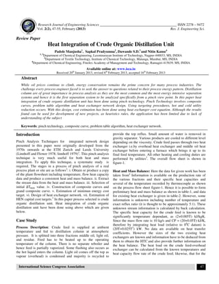
Process Description: Crude feed is supplied at ambient
temperature and fed to distillation column at atmospheric
pressure. It is splitted into three fractions middle oil, light oil,
and residue. Feed has to be heated up to the operating
temperature of the column. There is no separate reboiler and
hence feed is partially vaporized. Some flashing also occurs as
the hot liquid enters the column. Light oil comes off the top as
vapour (overhead) is condensed and majority is recycled to
provide the top reflux. Small amount of water is removed in
gravity separator. Various products are cooled to different level
depending on the viscosity. Crude feed passes through two heat
exchanger i.e.by overhead heat exchanger and middle oil heat
exchanger before entering a furnace which brings it up to its
final feed temperature. All other heating and cooling duties are
performed by utilities3
. The overall flow sheet is shown in
figure-1.
Heat and Mass Balance: Here the data for given work has been
taken from4
Information is available on the production rate of
the various fractions and their specific heat capacities and
several of the temperature recorded by thermocouple as shown
on the process flow sheet figure-1. Hence it is possible to form
preliminary heat and mass balance as shown in table-1, and data
for existing heat exchanger is given in table-2. However, some
information is unknown including number of temperature and
exact reflux ratio (it is thought to be approximately 5:1). These
unknown stream information is calculated by back calculation.
The specific heat capacity for the crude feed is known to be
significantly temperature dependant, as (2+0.005T) kJ/kgK.
Since the mass flow rate is 10 kg/s and CP = (20+0.05T) kJ/K,
therefore by integrating heat load (relative to 00
C datum) is
(20T+0.025T2
) kW. No data are available on heat transfer
coefficients. However the sizes of the two existing heat
exchangers are known and information have to be deduced from
them to obtain the HTC and also provide further information on
the heat balance. The heat load on the crude feed-overhead
exchanger can be calculated from the known temperatures and
heat capacity flow rate of the crude feed; likewise, that for the

2. Research Journal of Engineering Sciences___________
Vol. 2(2), 47-55, February (2013)
International Science Congress Association
middle oil-crude feed exchanger can be calculated from the
details of the middle oil, and the exit temperature of the crude
feed can then be back calculated as 920
C. Heat loads are
calculated as given below,

3. ∆
10

4. 2.1

5. 60 20 880.
Here value of Cp is taken from 2+0.005T. T is
temperature of inlet and outlet cold fluid temperature. Heat load
for the second heat exchanger is calculated from hot fluid i.e.
middle oil.

6. ∆
5

7. 2

8. 199 123 760.
The overall heat transfer coefficients U for the exchangers are
then calculated to be 0.2 and 0.125kW/m2
K, respectively. The
basic relationship of U to the film heat transfer coefficients h
(ignoring fouling and wall resistance) is:
Existing flow sheet for Crude
_________________________________________________
International Science Congress Association
crude feed exchanger can be calculated from the
etails of the middle oil, and the exit temperature of the crude
C. Heat loads are
Here value of Cp is taken from 2+0.005T. T is the mean
temperature of inlet and outlet cold fluid temperature. Heat load
for the second heat exchanger is calculated from hot fluid i.e.
the exchangers are
K, respectively. The
basic relationship of U to the film heat transfer coefficients h
#
$
#
%
'
#
%(
Assuming that all organic liquids have the same film HTC,
setting h1 = h2 for the crude feed/middle oil exchanger gives h
as 0.25 kW/m2
K. Back calculation for the crude feed/overheads
exchanger gives a film HTC of 1kW/m
for the condensing stream as shown in Tab
condensing overheads over this range can be calculated as
80kW/K.
CP (kW/K) =
)
∆*
CP (kW/K) =
++,
#-./##-
= 80kW/K.
Measurements of cooling water flow and temperature drop
indicate that the heat load on the following overheads cooler is
1.8 MW, and since the temperature drop is 60
of 30kW/K. The current level of heat recovery in these two
exchangers is 1640kW .
Figure-1
Existing flow sheet for Crude Distillation Unit
_____________ ISSN 2278 – 9472
Res. J. Engineering Sci.
48
uids have the same film HTC,
for the crude feed/middle oil exchanger gives h
K. Back calculation for the crude feed/overheads
exchanger gives a film HTC of 1kW/m2
K, which is reasonable
for the condensing stream as shown in Table-2. The Cp for the
condensing overheads over this range can be calculated as
= 80kW/K.
Measurements of cooling water flow and temperature drop
the following overheads cooler is
1.8 MW, and since the temperature drop is 60o
C this gives a CP
of 30kW/K. The current level of heat recovery in these two

9. Research Journal of Engineering Sciences________________________________________________________ ISSN 2278 – 9472
Vol. 2(2), 47-55, February (2013) Res. J. Engineering Sci.
International Science Congress Association 49
Stream Data Extraction: With consistent heat and mass
balance available, stream data are extracted. Here only those
flows which require heating or cooling are extracted from given
process. Therefore, the light oil and water from the separator are
ignored. The overheads emerging from the separator are mixed
directly with fresh oil and direct heat exchange of 100 kW takes
place. The amount of heat involved in these two streams is so
small and the temperature so low that they can be safely
ignored. This leaves five actual streams whose characteristics
are listed in table-3. From above table it has been found that
total heat load for the cold streams is 8500kW and for the hot
streams is 5000kW. The current level of heat recovery observed
is 1640kW. This implies that current hot utility and cold utility
demands are 6860kW and 3360kW respectively. For reducing
the hot utility and cold utility demand targeting procedure is
applied. There are two targeting procedure applied for utility
reduction. One is to draw “composite curve” and other is to
form “problem table algorithm”. For drawing the composite
curve, understanding of pinch concept is very essential.
Pinch Analysis Review
Introduced by Linnhoff et al. pinch analysis has a purpose to
identify the optimum heat recovery of process and to establish
the most promising options concerning cost of the heat
exchanger network (HEN). The identification of possible
opportunities of thermal integration can be visualized through
the hot and cold composite curves (CCs), as shown in figure-2.5
Composite curve: These are combinations of the thermal
streams of total process, in terms of their heat contents over
each temperature level (temperature × enthalpy). Here minimum
temperature difference is taken as 20o
C and data for actual and
shifted temperature curve is given in table-4. Hot and cold
composite curves are drawn using data given in table-5. Hot and
cold composite curves represent the energy avaibility and the
requirement of the overall process respectively. Their
overlapping indicates the maximum heat recovery of process,
whereas the overshoot determines the minimum hot and cold
utility requirements of the process (targets). The minimum
temperature difference (∆T), with regard to capital cost is the
limit for the approximation between the curves and limit
imposed by the project i.e. the pinch point. In application terms
it is relevant to observe that there should be no heat transfer
across the pinch, because transfer of heat indicates an increase
in hot and cold utilities6
.
Table-1
Heat and Mass balance for organic process
Flow stream
Production
Rate
(ton/hr)
Mass
flow
(kg/s)
Specific heat
(kJ/kgK)
Heat capacity
rate(kW/K)
Initial
temperature
(o
c)
Final
temperature
(o
c)
Heat Load
(kW)
Crude feed 36 10 2+0.05T 25 20 180 4000
Dehydrate ? (9.67) 3.1 30 152 302 4500
Bottoms 14.4 4 2.5 10 261 158 1030
Middle oil 18 5 2 10 199 70 1290
Light oil 9.6 2.67 2 5.33 52 52 0
Overheads ? ? ? ? 112 45 ?
Fresh oil 7.2 2 2 4 20 45 100
Water 1.2 0.33 4.19 1.4 52 52 0
Here question marks denote unknown values and bracketed values were found by back calculation
Table-2
Data for existing Heat Exchangers
Streams
Exchanger area
(m2
)
Hot stream
temperature (o
C)
Cold stream
temperature (o
C)
Log mean
temperature
difference (o
C)
Calculated heat
load
(kW)
Calculated
overall HTC
(kW/01
K)
CF/Ohds 57.5 123-112 20-60 77 880 0.2
CF/MO 73.2 199-123 60-(92) 83 760 0.125
Table-3
Stream data extraction
Stream name Stream type
Initial
temperature (o
C)
Target
temperature (o
C)
Film HTC
(kW/01K)
Heat capacity
flow rate (kW/K)
Heat flow rate
(kW)
Bottoms Hot 1 261 158 0.25 10 1030
Middle Oil Hot 2 199 70 0.25 10 1290
Overheads Hot 3A 123 112 1 80 880
Hot 3B 112 52 1 30 1800
Crude Feed Cold 1 20 180 0.25 20+0.05T -4000
Dehydrate Cold 2 152 302 0.25 30 -4500

10. Research Journal of Engineering Sciences___________
Vol. 2(2), 47-55, February (2013)
International Science Congress Association
Actual and shifted temperature for given stream extracted
Stream
Name
Actual Temperature
Heat
capacity
Cp(kW/K)
Inlet Temperature
(o
C)
Hot 1 10 261
Hot 2 10 199
Hot 3A 80 123
Hot 3B 30 112
Cold 1 20+0.005T 20
Cold 2 30 152
Data required for plotting the composite curves.
Actual
Temperature(o
C)
Heat
capacity(kW/K)
261
10
199
20
158
10
123
90
112
40
70
30
52
0
50
100
150
200
250
300
350
0 5000 10000
Actual
Temperature(oC)
Heat Flow(KW)
COMPOSITE CURVES
Black
Grey
_________________________________________________
International Science Congress Association
Table-4
Actual and shifted temperature for given stream extracted
Actual Temperature Shifted Temperature
Inlet Temperature Outlet
Temperature(o
C)
Heat
capacity
Cp(kW/K)
Inlet Temperature
(o
C)
158 10 251
70 10 189
112 80 112
52 30 102
180 20+0.005T 30
302 30 162
Table-5
Data required for plotting the composite curves.
Enthalpy(kW)
Shifted
Temperature(o
C)
Heat
capacity(kW/K)
251
620 10
189
820 20
148
350 10
113
990 90
102
1680 40
60
540 30
42
Figure-2
Composite curve
0
50
100
150
200
250
300
350
0 5000
Shifted
Temperature(oC)
Heat Flow(KW)
COMPOSITE CURVES
15000
COMPOSITE CURVES
Black--HCC
Grey--CCC
_____________ ISSN 2278 – 9472
Res. J. Engineering Sci.
50
Shifted Temperature
Inlet Temperature
C)
Outlet
Temperature
(o
C)
251 148
189 60
112 102
102 42
30 190
162 312
Heat
capacity(kW/K)
Enthalpy(kW)
620
820
350
990
1680
540
10000 15000
Heat Flow(KW)
COMPOSITE CURVES

11. Research Journal of Engineering Sciences___________
Vol. 2(2), 47-55, February (2013)
International Science Congress Association
Composite curves for hot and cold fluid for actual and shifted
temperature are drawn using data shown in
Composite curves for actual temperature are shown in figure
2(a) and for shifted temperature are shown in figure 2(b). The
grand composite curve (GCC) shown in figure
also used in pinch analysis. This grand composite curve is
plotted using cascade figure-5 that combines hot and cold
composite curves in a single curve, also through the sum of their
heat content in each temperature level. For zero value of the
enthalpy (horizontal axis), the temperature of that point
coincides with the pinch point. Using GCC, it is easier to
observe that, in the temperature level above the pinch, the
process just needs hot utility, whereas below the pinch the
demand is for cold utility. In case of many utilities (multiple
_________________________________________________
International Science Congress Association
Composite curves for hot and cold fluid for actual and shifted
temperature are drawn using data shown in table-4 and 5.
Composite curves for actual temperature are shown in figure
2(a) and for shifted temperature are shown in figure 2(b). The
te curve (GCC) shown in figure-3 is another tool,
This grand composite curve is
5 that combines hot and cold
composite curves in a single curve, also through the sum of their
mperature level. For zero value of the
enthalpy (horizontal axis), the temperature of that point
coincides with the pinch point. Using GCC, it is easier to
observe that, in the temperature level above the pinch, the
below the pinch the
demand is for cold utility. In case of many utilities (multiple
level utilities), it is possible to choose one of them, based on the
closer temperature level to the demand, minimizing the heat
transfer irreversibility. GCC also shows th
which is able to generate power using the degradation from high
to low steam pressure. From this GCC, location of the pinch has
been identified. At temperature 113
at which there is no heat transfer. Comp
same value as in problem table algorithm. It gives simple
framework for numerical analysis. The cold utility target
utility target should equal the bottom line of the infeasible heat
cascade which is 3535.35kW. These calculation
cross-checks that the stream data and heat cascades have been
evaluated correctly 7
.
Figure-3
Grand Composite Curve
Figure-4
Stream and Temperature Intervals
_____________ ISSN 2278 – 9472
Res. J. Engineering Sci.
51
level utilities), it is possible to choose one of them, based on the
closer temperature level to the demand, minimizing the heat
transfer irreversibility. GCC also shows the use of steam turbine
which is able to generate power using the degradation from high
to low steam pressure. From this GCC, location of the pinch has
been identified. At temperature 113o
C pinch temperature occurs
at which there is no heat transfer. Composite curve shows the
same value as in problem table algorithm. It gives simple
framework for numerical analysis. The cold utility target - Hot
utility target should equal the bottom line of the infeasible heat
cascade which is 3535.35kW. These calculations provide useful
checks that the stream data and heat cascades have been

12. Research Journal of Engineering Sciences________________________________________________________ ISSN 2278 – 9472
Vol. 2(2), 47-55, February (2013) Res. J. Engineering Sci.
International Science Congress Association 52
The Problem Table: Composite curve requires a graph paper
and scissor approach (for sliding the graph relative to one
another which would be messy and imprecise. Therefore, we are
using an algorithm for setting the target algebraically “The
problem table”. Following steps are to be done for the formation
of the problem table 8
. i. Enthalpy balance interval was set up
based on stream supply and target temperature shown in figure-
4, ii. The same is to be done for hot and cold stream together to
allow for the maximum possible amount of heat exchange with
each temperature interval. iii. The modification needed here is
that within any interval hot and cold stream are at least ∆T
apart. iv. This is done by using shifted temperature which is set
at 1/2∆T below hot stream temperature and 1/2∆T above
cold stream temperature. v. Now set the shifted temperature of
stream in a descending order from (higher to lower). vi. Setting
up the interval in this way guarantees that full heat interchange
within any interval is possible. vii. Each interval will have either
a net surplus or net deficit of heat as dictated by enthalpy
balance. viii. Enthalpy balance can easily be calculated for each
according to ∆23 45 46# ∑CP%:; ≤ ∑CP=:?.
In table-6, it is indicated that last column indicates whether an
interval is in heat surplus or heat deficit. Therefore it would be
possible to produce a feasible network design based on the
assumption that (a) all surplus intervals rejected heat to cold
utility. (b) all deficit intervals took heat from hot utility.
However this would not be very sensible because it would
involve rejecting and accepting heat at inappropriate
temperature. We have to exploit a key feature for the
temperature intervals. From figure-5(a), it is clearly seen that
from start there is negative flow of 1830kW, 1220 kW, 49.975
kW, 1046 kW.925 kW, 108.85 kW between interval 1-2,2-3,3-
4,4-5 is thermodynamically infeasible. To make it just equal to
zero, 4833.625kW of heat must be added from hot utility as
shown in figure-5(b) and cascaded right through the system. The
net result of this operation is that the maximum utilities
requirements have been predicted (i.e.4834kW hot and 1253kW
cold) 9
.
Heat Exchanger Network Design
For designing a heat exchanger network the most useful
representation is the “grid diagram” introduced by Linnhoff and
flower. The process streams are drawn as horizontal lines with
high temperature on the left and hot stream at the top.Cold
stream are drawn at bottom and flow from right to left. Streams
are represented by square boxes. Coolers and Heaters are
represented by circles (C) and (H). Heat exchangers which are
used to exchange the heat between the two process streams are
marked by two circles and two circles are connected by vertical
line. Two circles with vertical line connect the two streams
between which heat is being exchanged10
.
Table-6
Problem Table Algorithm (Temperature intervals and heat loads for above process)
@A (o
C) Interval No. Si-Si+1(o
C)
∑CPhot-∑CPcold
(kW/o
C)
∆HI(kW)
Surplus or
Deficit
S1=312
1 61 -30 -1830 Deficit
S2=251
2 61 -20 -1220 Deficit
S3=190
3 1 -49.475 -49.475 Deficit
S4=189
4 27 -38.775 -1046.925 Deficit
S5=162
5 14 -7.775 -108.85 Deficit
S6=148
6 35 -16.525 -578.375 Deficit
S7=113
7 11 64.625 710.875 Surplus
S8=102
8 42 15.95 669.9 Surplus
S9=60
9 18 7.45 134.1 Surplus
S10=42
10 12 -21.8 -261.6 Surplus
S11=30

13. Research Journal of Engineering Sciences___________
Vol. 2(2), 47-55, February (2013)
International Science Congress Association
The grid is much easier to draw than a flow sheet, especially as
heat exchangers can be placed in any order without redrawing
the stream system. Also, the grid represents the countercurrent
nature of the heat exchange, making it easier to
temperature feasibility. Finally, the pinch is easily represented
in the grid, whereas it cannot be represented on the flow sheet.
For drawing a grid diagram, above the pinch,
below the pinch, ∑CP%:; B ∑CP=:?. Heat excha
design for given process is shown in figure-6. From above grid
diagram, heat exchanger, heater, cooler summery is given in
table-7 and 8. From grid diagram according to rules, we need
total 4 heat exchangers, 2 heaters and 2 coolers. Initially
two heat exchangers have been used heat recovery was around
(a)Infeasible (b) Feasible
_________________________________________________
International Science Congress Association
The grid is much easier to draw than a flow sheet, especially as
heat exchangers can be placed in any order without redrawing
the stream system. Also, the grid represents the countercurrent
nature of the heat exchange, making it easier to check exchanger
temperature feasibility. Finally, the pinch is easily represented
in the grid, whereas it cannot be represented on the flow sheet.
∑CP%:; ≤ ∑CP=:?
. Heat exchanger network
6. From above grid
heat exchanger, heater, cooler summery is given in
8. From grid diagram according to rules, we need
total 4 heat exchangers, 2 heaters and 2 coolers. Initially when
two heat exchangers have been used heat recovery was around
1640kW but by using 4 heat exchangers in this modified
process, heat recovery is about 3860kW. And for modified
process area requirement is 545.6m
hot utility and cold utility has been calculated as given below.
%HUR =
D+D,/E+...D.
D+D,
×100 = 29.5%
%CUR =
..D,/#-F.
..D,
×100 = 62.7%
In these existing organic distillation processes, hot and cold
utility requirement decreases but number of exchanger increases
as shown in following grid figure-6.
(a)Infeasible (b) Feasible
Figure-5
Infeasible and feasible heat cascades
_____________ ISSN 2278 – 9472
Res. J. Engineering Sci.
53
1640kW but by using 4 heat exchangers in this modified
process, heat recovery is about 3860kW. And for modified
m-
. Percentage reduction in
old utility has been calculated as given below.
×100 = 29.5%
×100 = 62.7%
In these existing organic distillation processes, hot and cold
utility requirement decreases but number of exchanger increases
6.

14. Research Journal of Engineering Sciences________________________________________________________ ISSN 2278 – 9472
Vol. 2(2), 47-55, February (2013) Res. J. Engineering Sci.
International Science Congress Association 54
Figure-6
Combined heat exchanger grid diagram
Tabel-7
Heat Exchanger Summery
HEX No.
Thi
(o
C)
Tho
(o
C)
Tci
(o
C)
Tco
(o
C)
Heat Load
(KW)
Area
(m2)
1 199 123 103 133.4 760 158.4
2 261 158 103 174.6 1030 118.5
3 123 112 67.8 103 880 144.2
4 112 72 20 67.8 1195 124.5
Table-8
Heaters and Coolers summery
Heater No. Tci(o
C) Tco (0
C) CPc Heat Load(KW)
1 174 180 25 135
2 152 302 30 4497
Cooler No. Thi(0
C) Tho(0
C) CPh Heat Load(KW)
1 123 70 10 530
2 72 52 30 604
Table-9
Comparison of targets with current energy use
Situation ∆Tmin value (0
C) HU(KW) CU(KW)
Heat
recovery(KW)
Exchanger
Area(m2)
Current 63 6860 3360 1640 130.7
Target 20 4834 1253 3865 545.6
Cost Estimation
The final information is to be collected is the cost of heating and
cooling and the capital cost of new heat exchangers11
. In this
process, the hours worked per year are also needed i.e. here the
figure is 5000. Heating is provided in the coal fired furnace
whose mean temperature is approximately 4000
C. The fuel costs
$72/ton. Gross calorific value is 28.8 GJ/ton. Gross efficiency is
75%. Useful heat delivered cost is $3.33/GJ or $12 /MW.
Cooling is much cheaper, cooling water is recirculated to a
cooling tower which works in the range 25-35o
C. Now
exchanger cost is given by the following formula,
GHIℎKLMNO
PQR$ T ' KUV
The coefficients for heat exchanger cost are a=300, b=0.95,
d=10000 for cooler d=5000and are given in dollar($).Total
energy cost is given by,
G
$ W Q$

15. C$
$
$Y#
Hen Total Capital Cost Targeting
Here the targets for the minimum surface area (U) and the
number of units (Z) can be combined together with the heat

16. Research Journal of Engineering Sciences________________________________________________________ ISSN 2278 – 9472
Vol. 2(2), 47-55, February (2013) Res. J. Engineering Sci.
International Science Congress Association 55
exchanger cost law to determine the targets for the HEN capital
cost
[]. Capital cost is annualized using an annualization
factor that takes into account interest payments on borrowed
capital. The equation used for calculating the total capital cost
and exchanger cost law is given below12
$[] ^Z _K ' V `
U
Z
a
b
cd
ef
' ^Z _K ' V `
U
Z
a
b
cd
gf
Where a, b, c are constants in exchanger cost law. Z is
calculated by,
Z hZ ' Zb ' Zi 1jef + hZ + Zb + Zi − 1jgf
Z is found to be 8 and U is 546m2
. Consider carbon steel
shell and tube heat exchangers. For this, constants are a=16000;
b=3200; c=0.7. and
($)[] is found to be 619626.5$.
Generally installed cost can be considered 3.5 times the
purchase cost. In this way heat exchanger capital cost and
installed cost is to be calculated before and after heat
integration.
Conclusion
In present study using pinch technology for heat integration of
organic distillation unit, heat recovery of 3865kW occurs. Hot
utility reduction is around 30% of the total heat load while the
cold utility reduction is around 63% of the initial cold utility
demand. Minimum number of units for heat transfer i.e. heater,
cooler and heat exchangers increase, thereby capital cost
increase is around 58% of the initial capital cost. As capital cost
investment is one time investment, it is beneficial to use pinch
technology. Table-8 shows the result for cost of heat exchanger
before and after heat integration in the present study.
References
1. Linnhoff B., Townsend D.W., Boland D. et al., A User
Guide to Process Integration For The efficient Use of
Energy, I. Chem E, UK (1982)
2. Ian C. Kemp, Pinch analysis and Process Integration: a user
guide on process integration for the efficient use of energy,
second edition, Elsevier, Butterworth-Heinemann, UK
(2007)
3. Robin Smith, Chemical Process Design, McGraw-Hill,
New York (1995)
4. Linnhoff B., Mason D.R. and Wardate I., Understanding
Heat Exchanger Networks, Computer and Chemical
Engineering, (1979)
5. Marechal F. and Kalitventzeff B., A new graphical
Technique for evaluating the integration of utility systems,
Computers and Chemical Engineering, 20 (1996)
6. Linnhoff B., Don U.K. and Vredeveld R., Pinch Technology
Has Come of Age, Chemical Engineering Progress, (1984)
7. Polley G.T. and Heggs P.J., Don't let the Pinch Pinch You,
Chemical Engineering Progress, (27-36), December, (1999)
8. Ahmad S. and Hui D.C.W., Heat recovery between areas of
integrity, Computer Chemical Engineering, 15(12), 809-832
(1991)
9. Linnhoff B. and Polley G.T. and Sahdev V., Linnhoff March
Ltd., U.K., General Process Improvements Through Pinch
Technology, Chemical Engineering Progress, (1988)
10. Linnhoff B. and Hindumarsh E., The pinch design method of
heat exchanger networks, Chemical Engineering. Science,
38(5), 745-763 (1983)
11. Mishra A.K., Nawal S. and Thundil Karuppa Raj R., Heat
Transfer Augmentation of Air Cooled Internal Combustion
Engine Using Fins through Numerical Techniques,
Research J. Engineering Sci., 1(2), 32-40 (2012)
12. Heggs P.J., Minimum temperature difference approach
concept in heat exchanger networks, J Heat Recovery Systems
CHP, 9(4), 367-375 (1989)