Series(ベクトル)
>>> a =pd.Series(range(5), index=list(“abcde”)) # 0..5のリストにa..eのインデックス
>>> a[list(“ace”)] #indexアクセス
a 0
c 2
e 4
dtype: int64
>>> a[[0,2,4]] # 0,2,4番目の要素
a 0
c 2
e 4
dtype: int64
>>> a[(a<1)|(a>3)] #1より小さい、または3より大きい要素
a 0
e 4
dtype: int64
pychembldb
from pychembldb import*
#Inhibition of recombinant Syk
#Bioorg. Med. Chem. Lett. (2009) 19:1944-1949
assay = chembldb.query(Assay).filter_by(chembl_id="CHEMBL1022010").one()
for act in assay.activities:
if act.standard_relation == "=":
print act.compound.molecule.structure.molfile, "n$$$$"
先に使ったSYKのデータから
sdfを作っておく


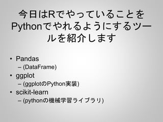

![Series(ベクトル)
>>> a = pd.Series(range(5), index=list(“abcde”)) # 0..5のリストにa..eのインデックス
>>> a[list(“ace”)] #indexアクセス
a 0
c 2
e 4
dtype: int64
>>> a[[0,2,4]] # 0,2,4番目の要素
a 0
c 2
e 4
dtype: int64
>>> a[(a<1)|(a>3)] #1より小さい、または3より大きい要素
a 0
e 4
dtype: int64](https://image.slidesharecdn.com/pandas-140704062322-phpapp02/85/R-Python-11-320.jpg)
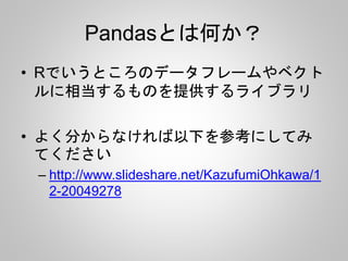
![DataFrameを作成
>>> pd.DataFrame([[1,2,3],[4,5,6]])
0 1 2
0 1 2 3
1 4 5 6](https://image.slidesharecdn.com/pandas-140704062322-phpapp02/85/R-Python-12-320.jpg)
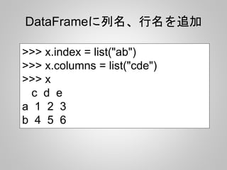
![DataFrameの列にアクセス
>>> x["c"]
a 1
b 4
Name: c, dtype: int64
>>> x.c
a 1
b 4
Name: c, dtype: int64](https://image.slidesharecdn.com/pandas-140704062322-phpapp02/85/R-Python-14-320.jpg)
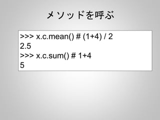
![データフレームの結合
>>> x
0 1
0 1 0
1 -2 3
>>> pd.concat([x, x], axis=0) # rbind
0 1
0 1 0
1 -2 3
0 1 0
1 -2 3
>>> pd.concat([x, x], axis=1) # cbind
0 1 0 1
0 1 0 1 0
1 -2 3 -2 3](https://image.slidesharecdn.com/pandas-140704062322-phpapp02/85/R-Python-16-320.jpg)


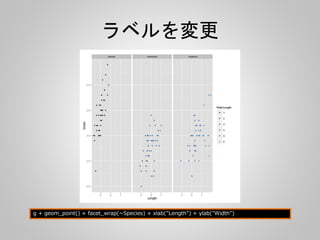
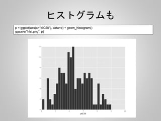
![pandasで読み込んでggplotで描画
import pandas as pd
from ggplot import *
import numpy as np
d = pd.read_csv("syk.csv")
d["pIC50"] = 9 - np.log10(d["IC50"])
p = ggplot(aes(x='MWT', y='ALOGP', color="pIC50", size="pIC50"), data=d) + geom_point()
#print p
ggsave("2dplot.png", p)](https://image.slidesharecdn.com/pandas-140704062322-phpapp02/85/R-Python-30-320.jpg)


![PCA
from rdkit import Chem
from rdkit.Chem import AllChem, DataStructs
from sklearn.decomposition import PCA
from ggplot import *
import numpy as np
import pandas as pd
suppl = Chem.SDMolSupplier('syk.sdf')
fps = []
for mol in suppl:
fp = AllChem.GetMorganFingerprintAsBitVect(mol, 2)
arr = np.zeros((1,))
DataStructs.ConvertToNumpyArray(fp, arr)
fps.append(arr)
Morganフィンガープリントを作って
Scikit-learnで扱えるように
NumpyArrayに変換](https://image.slidesharecdn.com/pandas-140704062322-phpapp02/85/R-Python-41-320.jpg)
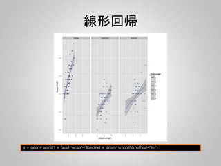
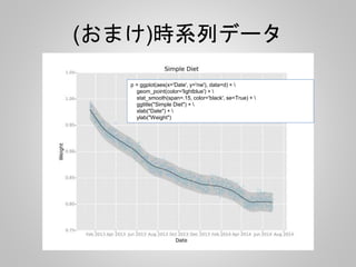
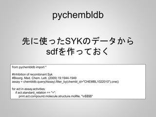
![PCA
pca = PCA(n_components=2)
pca.fit(fps)
v = pca.components_
d = pd.DataFrame(v).T
d.columns = ["PCA1", "PCA2"]
g = ggplot(aes(x="PCA1", y="PCA2"), data=d) + geom_point(color="lightblue") + xlab("PCA1") +
ylab("PCA2")
ggsave("pca.png", g)
PCAで第二主成分まで計算して、
Xに第一、Yに第二主成分をプロット](https://image.slidesharecdn.com/pandas-140704062322-phpapp02/85/R-Python-42-320.jpg)

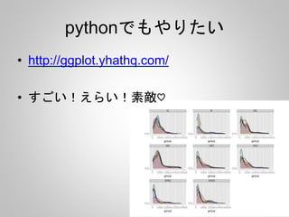
![RandamForest
from rdkit import Chem
from rdkit.Chem import AllChem, DataStructs
from sklearn import cross_validation
from sklearn.ensemble import RandomForestClassifier
import numpy as np
import pandas as pd
d = pd.read_csv("syk.csv")
d["pIC50"] = 9 - np.log10(d["IC50"])
d["ACT"] = d.pIC50.apply(lambda x: 1 if x > 8 else 0)
先に使ったSYKのデータpIC50をもとめて
8オーダーより強いものを活性ありとした
(0:活性あり、1:活性なし)](https://image.slidesharecdn.com/pandas-140704062322-phpapp02/85/R-Python-45-320.jpg)
![RandamForest
suppl = Chem.SDMolSupplier('syk.sdf')
fps = []
for mol in suppl:
fp = AllChem.GetMorganFingerprintAsBitVect(mol, 2)
arr = np.zeros((1,))
DataStructs.ConvertToNumpyArray(fp, arr)
fps.append(arr)
RDKitでsdfを読み込みMorganFingerprint
を計算し、それをScikit-learnで使えるように
NumpyArrayに変換](https://image.slidesharecdn.com/pandas-140704062322-phpapp02/85/R-Python-46-320.jpg)
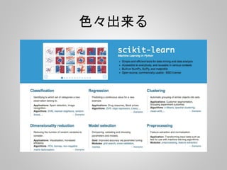
![RandamForest
x_train, x_test, y_train, y_test = cross_validation.train_test_split(fps, d, test_size=0.4,
random_state=0)
print x_train.shape, y_train.shape
print x_test.shape, y_test.shape
rf = RandomForestClassifier(n_estimators=100, random_state=1123)
rf.fit(x_train, y_train[:,5])
print "predictn", rf.predict(x_test)
print "nresultn", y_test[:,5]
#print y_test[:,[0,5]]
データを訓練、テストセットにわけ、
RandamForestでモデルをつくり
テスト](https://image.slidesharecdn.com/pandas-140704062322-phpapp02/85/R-Python-47-320.jpg)
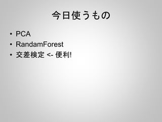
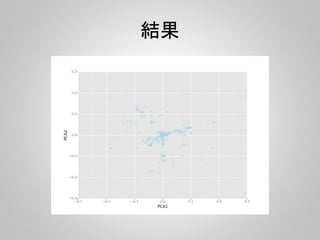
![Result
predict
[0 0 0 0 0 1 0 0 0 0 0 0 0 0 0 0 0 0 1 0 0 0 0 1 0 0 1 0 0 0 0 0 0 0 0 0 0 0 0 0
0 1 0 0 0 0 0 0 0 0 0 0 0 0 0 0 0]
result
[0 0 0 0 0 1 0 0 0 0 0 0 0 0 0 0 0 0 0 0 0 0 0 1 1 0 1 0 0 0 0 0 0 0 0 0 0 0 0 0
0 1 0 0 0 0 0 0 0 0 0 0 0 0 0 0 0]](https://image.slidesharecdn.com/pandas-140704062322-phpapp02/85/R-Python-48-320.jpg)


![[機械学習]文章のクラス分類](https://cdn.slidesharecdn.com/ss_thumbnails/ss-160218112331-thumbnail.jpg?width=640&height=640&fit=bounds)