7.2.1.mk_imlist.py
imlist =sorted(imtools.get_imlist('first1000'))
nbr_images = len(imlist)
featlist = [imlist[i][:-3]+'sift' for i in range(nbr_images)]
!
with open('ukbench_imlist.pkl','wb') as f:
pickle.dump(imlist,f)
pickle.dump(featlist,f)
!
with open('webimlist.txt','w') as f:
for i in imlist:
f.write(i)
f.write('n')
ボキャブラリ作成の前に二つのリストをファイルに書き出して置く必要があります。
11.
7.2.1 ボキャブラリの作成
7.2.1.mk_sift.py
import imtools
import sift
!
imlist = imtools.get_imlist('first1000')
nbr_images = len(imlist)
featlist = [ imlist[i][:-3]+'sift' for i in range(nbr_images)]
!
for i in range(nbr_images):
sift.process_image(imlist[i],featlist[i])
featlist: 拡張子をsiftにした画像ファイル名のリスト。実行すると処理の後この
リストのファイルが生成されます。
SIFTアルゴリズムの処理はPythonではなく、
VLFeatのバイナリが行います。
12.
7.2.1 vocabulary.py
classVocabulary(object):
!
def __init__(self,name):
self.name = name
self.voc = []
self.idf = []
self.trainingdata = []
self.nbr_words = 0
!
def train(self,featurefiles,k=100,subsampling=10):
nbr_images = len(featurefiles)
descr = []
descr.append(sift.read_features_from_file(featurefiles[0])[1])
descriptors = descr[0] #stack all features for k-means
for i in arange(1,nbr_images):
descr.append(sift.read_features_from_file(featurefiles[i])[1])
descriptors = vstack((descriptors,descr[i]))
!
self.voc,distortion = kmeans(descriptors[::subsampling,:],k,1)
self.nbr_words = self.voc.shape[0]
imwords = zeros((nbr_images,self.nbr_words))
for i in range( nbr_images ):
imwords[i] = self.project(descr[i])
!
nbr_occurences = sum( (imwords > 0)*1 ,axis=0)
!
self.idf = np.log( (1.0*nbr_images) /
(1.0*nbr_occurences+1) )
self.trainingdata = featurefiles
!
def project(self,descriptors):
""" 記述子をボキャブラリに射影して、
単語のヒストグラムを作成する """
!
# ビジュアルワードのヒストグラム
imhist = zeros((self.nbr_words))
words,distance = vq(descriptors,self.voc)
for w in words:
imhist[w] += 1
!
return imhist
scipy.cluster.vqのk平均実装を利用、
行列形式の特徴量がk個にクラスタリングされます。
13.
7.2.1.mk_voc.py
import imtools
#imlist = sorted(imtools.get_imlist('first1000'))
imlist = imlist[:100] # for small memory
!
import pickle
import vocabulary
!
nbr_images = len(imlist)
featlist = [ imlist[i][:-3]+'sift' for i in range(nbr_images) ]
!
voc = vocabulary.Vocabulary('ukbenchtest')
voc.train(featlist,1000,10)
!
# ボキャブラリを保存する
with open('vocabulary.pkl', 'wb') as f:
pickle.dump(voc,f)
print 'vocabulary is:', voc.name, voc.nbr_words
ファイルをしぼらないと無理かも
7.3.1 データベースを設定する
imagesearch.py
def create_tables(self):
""" データベースのテーブルを作成する """
self.con.execute('create table imlist(filename)')
self.con.execute('create table imwords(imid,wordid,vocname)')
self.con.execute('create table imhistograms(imid,histogram,vocname)')
self.con.execute('create index im_idx on imlist(filename)')
self.con.execute('create index wordid_idx on imwords(wordid)')
self.con.execute('create index imid_idx on imwords(imid)')
self.con.execute('create index imidhist_idx on imhistograms(imid)')
self.db_commit()
3つのテーブルとインデクスを作成
16.
7.3.2.mk_index.py
import imtools
imlist = sorted(imtools.get_imlist('first1000'))
!
import pickle
import sift
import imagesearch
!
nbr_images = len(imlist)
featlist = [ imlist[i][:-3]+'sift' for i in
range(nbr_images)]
!
# ボキャブラリを読み込む
with open('vocabulary.pkl', 'rb') as f:
voc = pickle.load(f)
# Iedexerを生成する
indx =
imagesearch.Indexer('test.db',voc)
indx.create_tables()
!
# 画像を順番にボキャブラリに射影してデー
タベースに挿入する
for i in range(nbr_images):
locs,descr =
sift.read_features_from_file(featlist[i])
indx.add_to_index(imlist[i],descr)
!
# データベースをコミットする
indx.db_commit()
ボキャブラリを配列にもどす
17.
7.3.2 画像を追加する
defadd_to_index(self,imname,descr):
""" 画像と特徴量記述子を入力し、ボキャブラリに
射影して、データベースに追加する """
!
if self.is_indexed(imname): return
print 'indexing', imname
!
# 画像IDを取得する
imid = self.get_id(imname)
!
# ワードを取得する
imwords = self.voc.project(descr)
nbr_words = imwords.shape[0]
!
# 各ワードを画像に関係づける
for i in range(nbr_words):
1~30ぐらいまでのワードIDがimwordsに
insertされる。ワード=クラスターのID??
word = imwords[i]
# ワード番号をワードIDとする
self.con.execute("insert into imwords(imid,wordid,vocname)
values (?,?,?)", (imid,word,self.voc.name))
18.
7.3.2.query.py
from sqlite3import dbapi2 as sqlite
con = sqlite.connect('test.db')
print con.execute('select count (filename) from imlist').fetchone()
print con.execute('select * from imlist').fetchone()
!
実行すると下記のようにコンソールに表示される。
1,000件の画像が登録された?
(1000,)
(u’first1000/ukbench00000.jpg’,)
7.4.1 インデクスを用いて候補を取得する
特定のワードを含む画像を見つけるためにインデクスを利用しデー
タベースに問い合わせるだけで済むようになった。
Searcherクラスの定義つづき
def candidates_from_word(self,imword):
""" imwordを含む画像のリストを取得する """
!
im_ids = self.con.execute(
"select distinct imid from imwords where wordid=%d" % imword).fetchall()
return [i[0] for i in im_ids]
!
21.
7.4.1
Searcherクラスの定義つづき
defcandidates_from_histogram(self,imwords):
""" 複数の類似ワードを持つ画像のリストを取得する """
!
# ワードのIDを取得する
words = imwords.nonzero()[0]
!
# 候補を見つける
candidates = []
for word in words:
c = self.candidates_from_word(word)
candidates+=c
!
# 全ワードを重複なく抽出し、出現回数の大きい順にソートする
tmp = [(w,candidates.count(w)) for w in set(candidates)]
tmp.sort(cmp=lambda x,y:cmp(x[1],y[1]))
tmp.reverse()
!
# 一致するものほど先になるようにソートしたリストを返す
return [w[0] for w in tmp]
7.4.3 ベンチマークを測定し結果を描画する
defcompute_ukbench_score(src,imlist):
!
nbr_images = len(imlist)
pos = zeros((nbr_images,4))
# 各画像の検索結果の上位4件を得る
for i in range(nbr_images):
pos[i] = [w[1]-1 for w in src.query(imlist[i])[:4]]
!
# スコアを計算して平均を返す
score = array([ (pos[i]//4)==(i//4) for i in range(nbr_images)])*1.0
return sum(score) / (nbr_images)
検索結果の評価のために、検索結果の上位4件のうち、正解数の平均を返します。
※何が「正解」かは??同じモノを写した写真が4連番なことを利用しているのかも。


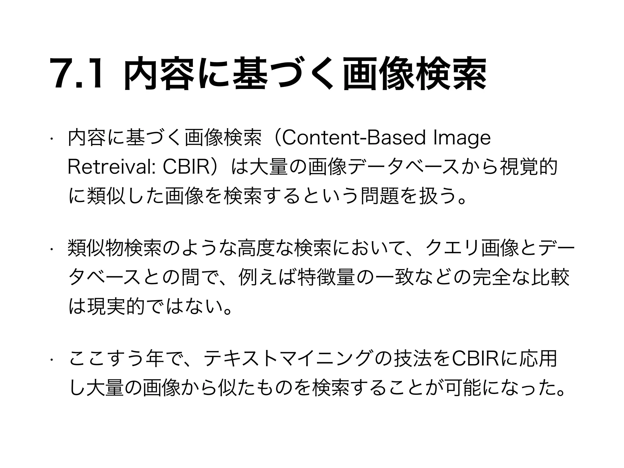
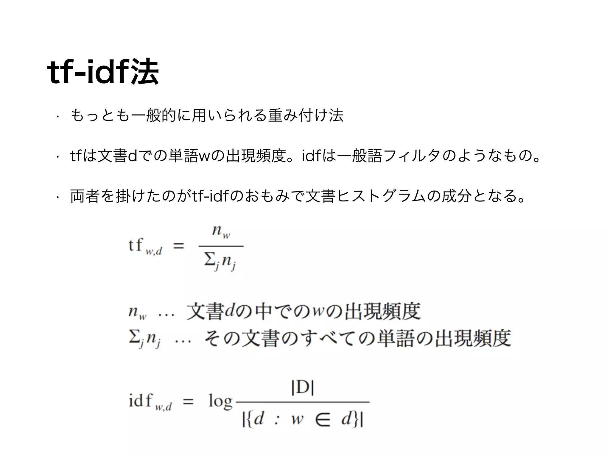
![tf-idf法の例
• 電気情報通信学会2006 [論文概要に対する色付き
アンダーライン付与システムの運用・分析]
http://www-kasm.nii.ac.jp/papers/takeda/05/
matsuoka06dews.pdf
• 全論文概要に含まれるキーワードに対する基準化
tfidf値のヒストグラム(図5)や全下線文に含まれ
るキーワードに対する基準化tfidf値のヒストグラム
(図6)のように利用される。](https://image.slidesharecdn.com/20148307-140829193229-phpapp02/75/7-_20140830-6-2048.jpg)

![7.2.1.mk_imlist.py
imlist = sorted(imtools.get_imlist('first1000'))
nbr_images = len(imlist)
featlist = [imlist[i][:-3]+'sift' for i in range(nbr_images)]
!
with open('ukbench_imlist.pkl','wb') as f:
pickle.dump(imlist,f)
pickle.dump(featlist,f)
!
with open('webimlist.txt','w') as f:
for i in imlist:
f.write(i)
f.write('n')
ボキャブラリ作成の前に二つのリストをファイルに書き出して置く必要があります。](https://image.slidesharecdn.com/20148307-140829193229-phpapp02/75/7-_20140830-10-2048.jpg)
![7.2.1 ボキャブラリの作成
7.2.1.mk_sift.py
import imtools
import sift
!
imlist = imtools.get_imlist('first1000')
nbr_images = len(imlist)
featlist = [ imlist[i][:-3]+'sift' for i in range(nbr_images)]
!
for i in range(nbr_images):
sift.process_image(imlist[i],featlist[i])
featlist: 拡張子をsiftにした画像ファイル名のリスト。実行すると処理の後この
リストのファイルが生成されます。
SIFTアルゴリズムの処理はPythonではなく、
VLFeatのバイナリが行います。](https://image.slidesharecdn.com/20148307-140829193229-phpapp02/75/7-_20140830-11-2048.jpg)
![7.2.1 vocabulary.py
class Vocabulary(object):
!
def __init__(self,name):
self.name = name
self.voc = []
self.idf = []
self.trainingdata = []
self.nbr_words = 0
!
def train(self,featurefiles,k=100,subsampling=10):
nbr_images = len(featurefiles)
descr = []
descr.append(sift.read_features_from_file(featurefiles[0])[1])
descriptors = descr[0] #stack all features for k-means
for i in arange(1,nbr_images):
descr.append(sift.read_features_from_file(featurefiles[i])[1])
descriptors = vstack((descriptors,descr[i]))
!
self.voc,distortion = kmeans(descriptors[::subsampling,:],k,1)
self.nbr_words = self.voc.shape[0]
imwords = zeros((nbr_images,self.nbr_words))
for i in range( nbr_images ):
imwords[i] = self.project(descr[i])
!
nbr_occurences = sum( (imwords > 0)*1 ,axis=0)
!
self.idf = np.log( (1.0*nbr_images) /
(1.0*nbr_occurences+1) )
self.trainingdata = featurefiles
!
def project(self,descriptors):
""" 記述子をボキャブラリに射影して、
単語のヒストグラムを作成する """
!
# ビジュアルワードのヒストグラム
imhist = zeros((self.nbr_words))
words,distance = vq(descriptors,self.voc)
for w in words:
imhist[w] += 1
!
return imhist
scipy.cluster.vqのk平均実装を利用、
行列形式の特徴量がk個にクラスタリングされます。](https://image.slidesharecdn.com/20148307-140829193229-phpapp02/75/7-_20140830-12-2048.jpg)
![7.2.1.mk_voc.py
import imtools
#imlist = sorted(imtools.get_imlist('first1000'))
imlist = imlist[:100] # for small memory
!
import pickle
import vocabulary
!
nbr_images = len(imlist)
featlist = [ imlist[i][:-3]+'sift' for i in range(nbr_images) ]
!
voc = vocabulary.Vocabulary('ukbenchtest')
voc.train(featlist,1000,10)
!
# ボキャブラリを保存する
with open('vocabulary.pkl', 'wb') as f:
pickle.dump(voc,f)
print 'vocabulary is:', voc.name, voc.nbr_words
ファイルをしぼらないと無理かも](https://image.slidesharecdn.com/20148307-140829193229-phpapp02/75/7-_20140830-13-2048.jpg)


![7.3.2.mk_index.py
import imtools
imlist = sorted(imtools.get_imlist('first1000'))
!
import pickle
import sift
import imagesearch
!
nbr_images = len(imlist)
featlist = [ imlist[i][:-3]+'sift' for i in
range(nbr_images)]
!
# ボキャブラリを読み込む
with open('vocabulary.pkl', 'rb') as f:
voc = pickle.load(f)
# Iedexerを生成する
indx =
imagesearch.Indexer('test.db',voc)
indx.create_tables()
!
# 画像を順番にボキャブラリに射影してデー
タベースに挿入する
for i in range(nbr_images):
locs,descr =
sift.read_features_from_file(featlist[i])
indx.add_to_index(imlist[i],descr)
!
# データベースをコミットする
indx.db_commit()
ボキャブラリを配列にもどす](https://image.slidesharecdn.com/20148307-140829193229-phpapp02/75/7-_20140830-16-2048.jpg)
![7.3.2 画像を追加する
def add_to_index(self,imname,descr):
""" 画像と特徴量記述子を入力し、ボキャブラリに
射影して、データベースに追加する """
!
if self.is_indexed(imname): return
print 'indexing', imname
!
# 画像IDを取得する
imid = self.get_id(imname)
!
# ワードを取得する
imwords = self.voc.project(descr)
nbr_words = imwords.shape[0]
!
# 各ワードを画像に関係づける
for i in range(nbr_words):
1~30ぐらいまでのワードIDがimwordsに
insertされる。ワード=クラスターのID??
word = imwords[i]
# ワード番号をワードIDとする
self.con.execute("insert into imwords(imid,wordid,vocname)
values (?,?,?)", (imid,word,self.voc.name))](https://image.slidesharecdn.com/20148307-140829193229-phpapp02/75/7-_20140830-17-2048.jpg)


![7.4.1 インデクスを用いて候補を取得する
特定のワードを含む画像を見つけるためにインデクスを利用しデー
タベースに問い合わせるだけで済むようになった。
Searcherクラスの定義つづき
def candidates_from_word(self,imword):
""" imwordを含む画像のリストを取得する """
!
im_ids = self.con.execute(
"select distinct imid from imwords where wordid=%d" % imword).fetchall()
return [i[0] for i in im_ids]
!](https://image.slidesharecdn.com/20148307-140829193229-phpapp02/75/7-_20140830-20-2048.jpg)
![7.4.1
Searcherクラスの定義つづき
def candidates_from_histogram(self,imwords):
""" 複数の類似ワードを持つ画像のリストを取得する """
!
# ワードのIDを取得する
words = imwords.nonzero()[0]
!
# 候補を見つける
candidates = []
for word in words:
c = self.candidates_from_word(word)
candidates+=c
!
# 全ワードを重複なく抽出し、出現回数の大きい順にソートする
tmp = [(w,candidates.count(w)) for w in set(candidates)]
tmp.sort(cmp=lambda x,y:cmp(x[1],y[1]))
tmp.reverse()
!
# 一致するものほど先になるようにソートしたリストを返す
return [w[0] for w in tmp]](https://image.slidesharecdn.com/20148307-140829193229-phpapp02/75/7-_20140830-21-2048.jpg)
![7.4.1.imagesearch.py
import sift
import imagesearch
!
execfile('loaddata.py')
!
!
src = imagesearch.Searcher('test.db',voc)
locs,descr = sift.read_features_from_file(featlist[0])
iw = voc.project(descr)
!
print 'ask using a histogram...'
print src.candidates_from_histogram(iw)[:10]
実行すると
(ワードID,ワード出現回数)のリストを作り、ソートします。
[655, 885, 96, 80, 871, 870, 645, 77, 886, 822]
処理結果は一致度の高い画像から順に並んだ画像IDのリストを返します。
ただし上位10件いずれも正しくありません。後の作業で検索結果を改善します。](https://image.slidesharecdn.com/20148307-140829193229-phpapp02/75/7-_20140830-22-2048.jpg)
![7.4.2 画像を用いて問い合わせる
Searcherクラスの定義つづき
def get_imhistogram(self,imname):
""" 画像のワードヒストグラムを返す """
im_id = self.con.execute(
"select rowid from imlist where filename='%s'" % imname).fetchone()
s = self.con.execute(
"select histogram from imhistograms where rowid='%d'" % im_id).fetchone()
!
# pickleを使って文字列をNumPy配列に変換する
return pickle.loads(str(s[0]))
ファイル名で指定されたヒストグラムをimhistogramsテーブルから読み込みます。](https://image.slidesharecdn.com/20148307-140829193229-phpapp02/75/7-_20140830-23-2048.jpg)
![7.4.2
Searcherクラスの定義つづき
def query(self,imname):
""" imnameの画像に一致する画像のリストを見つける """
!
h = self.get_imhistogram(imname)
candidates = self.candidates_from_histogram(h)
!
matchscores = []
for imid in candidates:
# 名前を取得する
cand_name = self.con.execute(
"select filename from imlist where rowid=%d" % imid).fetchone()
cand_h = self.get_imhistogram(cand_name)
cand_dist = sqrt( sum( (h-cand_h)**2 ) ) # L2距離を用いる
matchscores.append( (cand_dist,imid) )
!
# 距離の小さい順にソートした距離と画像IDを返す
matchscores.sort()
return matchscores](https://image.slidesharecdn.com/20148307-140829193229-phpapp02/75/7-_20140830-24-2048.jpg)
![7.4.2.query_by_image.py
import imagesearch
!
execfile('loaddata.py')
!
src = imagesearch.Searcher('test.db',voc)
print 'try a query...'
print src.query(imlist[0])[:10]
実行すると距離と画像IDから構成されるタプルのリストを返します。
try a query...
[(0.0, 1), (63.882705014737752, 2), (66.370174024180471, 3), (88.379861959611588, 560),
(88.831300789755403, 4), (90.46546302318913, 677), (90.912045406535654, 664),
(91.798692801150494, 672), (93.305948363435007, 670), (93.648278147545241, 659)]
!
距離は画像とワードのユークリッド距離を出力します。](https://image.slidesharecdn.com/20148307-140829193229-phpapp02/75/7-_20140830-25-2048.jpg)
![7.4.3 ベンチマークを測定し結果を描画する
def compute_ukbench_score(src,imlist):
!
nbr_images = len(imlist)
pos = zeros((nbr_images,4))
# 各画像の検索結果の上位4件を得る
for i in range(nbr_images):
pos[i] = [w[1]-1 for w in src.query(imlist[i])[:4]]
!
# スコアを計算して平均を返す
score = array([ (pos[i]//4)==(i//4) for i in range(nbr_images)])*1.0
return sum(score) / (nbr_images)
検索結果の評価のために、検索結果の上位4件のうち、正解数の平均を返します。
※何が「正解」かは??同じモノを写した写真が4連番なことを利用しているのかも。](https://image.slidesharecdn.com/20148307-140829193229-phpapp02/75/7-_20140830-26-2048.jpg)
![7.4.3.bench.py
import imagesearch
!
execfile('loaddata.py')
!
src = imagesearch.Searcher('test.db',voc)
!
#print imagesearch.compute_ukbench_score(src,imlist)
!
print imagesearch.compute_ukbench_score(src,imlist[:100])
実行すると
スコアは2.76となりました。
1000回の問い合わせは無理そうなので
画像を間引きます。](https://image.slidesharecdn.com/20148307-140829193229-phpapp02/75/7-_20140830-27-2048.jpg)
![7.4.3 ベンチマークを測定し結果を描画する
Searcherクラスの定義つづき。
検索結果を表示する関数を定義します。
def plot_results(src,res):
""" 検索結果リスト'res'の画像を表示する """
!
figure()
nbr_results = len(res)
for i in range(nbr_results):
imname = src.get_filename(res[i])
subplot(1,nbr_results,i+1)
imshow(array(Image.open(imname)))
axis('off')
show()](https://image.slidesharecdn.com/20148307-140829193229-phpapp02/75/7-_20140830-28-2048.jpg)
![7.4.3.plot.py
import imagesearch
!
execfile('loaddata.py')
!
src = imagesearch.Searcher('test.db',voc)
!
nbr_results = 6
res = [w[1] for w in src.query(imlist[0])[:nbr_results]]
imagesearch.plot_results(src,res)
引数resに任意の数の検索結果が渡ります。
plot_result()で結果が表示されます。
!
!
!](https://image.slidesharecdn.com/20148307-140829193229-phpapp02/75/7-_20140830-29-2048.jpg)
![7.4 配置を用いて結果をランキングする
7.4.rerank.py
# 画像リストとボキャブラリを読み込む
with open('ukbench_imlist.pkl','rb') as f:
imlist = pickle.load(f)
featlist = pickle.load(f)
!
nbr_images = len(imlist)
!
with open('vocabulary.pkl', 'rb') as f:
voc = pickle.load(f)
!
src = imagesearch.Searcher('test.db',voc)
!
# クエリ画像の番号と、検索結果の個数
q_ind = 38
nbr_results = 20
# 通常の検索
res_reg = [w[1] for w in src.query(imlist[q_ind])
[:nbr_results]]
print 'top matches (regular):', res_reg
!
# クエリ画像の特徴量を読み込む
q_locs,q_descr =
sift.read_features_from_file(featlist[q_ind])
q_locs[:,[0,1]] = q_locs[:,[1,0]]
fp = homography.make_homog(q_locs[:,:2].T)
!
# ホモグラフィーの対応付け用のRANSACモデル
model = homography.RansacModel()
rank = {}](https://image.slidesharecdn.com/20148307-140829193229-phpapp02/75/7-_20140830-30-2048.jpg)
![7.4.rerank.py
# 検索結果の画像特徴量を読み込む
for ndx in res_reg[1:]:
locs,descr =
sift.read_features_from_file(featlist[ndx-1])
locs[:,[0,1]] = locs[:,[1,0]]
!
# 一致度を調べる
matches = sift.match(q_descr,descr)
ind = matches.nonzero()[0]
ind2 = matches[ind]
tp = homography.make_homog(locs[:,:2].T)
!
# ホモグラフィーを計算し、インライアを数える。
# 一致度が足りなければ空リストを返す。
try:
H,inliers =
homography.H_from_ransac(fp[:,ind],tp[:,ind2],
model,match_theshold=4)
except:
inliers = []
# インライアの数を格納する
rank[ndx] = len(inliers)
!
# 最もモデルに当てはまるものが先頭になるよう
辞書をソートする
sorted_rank = sorted(rank.items(), key=lambda t:
t[1], reverse=True)
res_geom = [res_reg[0]]+[s[0] for s in
sorted_rank]
print 'top matches (homography):', res_geom
!
# 検索結果を描画する
imagesearch.plot_results(src,res_reg[:8])
imagesearch.plot_results(src,res_geom[:8])
7.4.rerank.pyの定義 続き](https://image.slidesharecdn.com/20148307-140829193229-phpapp02/75/7-_20140830-31-2048.jpg)