Predictive method in analyzing time trend in real production line on machine setup time. Well-known moving average and/or exponential smoothing techniques (method) to calculate the time reduction in production environment.

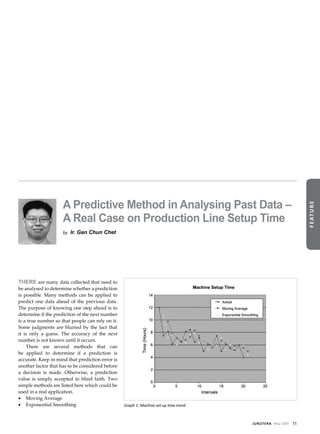
1. 11
Jurutera May 2009
A Predictive Method in Analysing Past Data –
A Real Case on Production Line Setup Time
by Ir. Gan Chun Chet
There are many data collected that need to
be analysed to determine whether a prediction
is possible. Many methods can be applied to
predict one data ahead of the previous data.
The purpose of knowing one step ahead is to
determine if the prediction of the next number
is a true number so that people can rely on it.
Some judgments are blurred by the fact that
it is only a guess. The accuracy of the next
number is not known until it occurs.
There are several methods that can
be applied to determine if a prediction is
accurate. Keep in mind that prediction error is
another factor that has to be considered before
a decision is made. Otherwise, a prediction
value is simply accepted in blind faith. Two
simple methods are listed here which could be
used in a real application.
• Moving Average
• Exponential Smoothing Graph 1: Machine set-up time trend
f
e
at
u
r
e

2. 12 May 2009 Jurutera
The two methods can be used in an
application where the next number
is required. Previously, I worked on
a project focusing on production line
setup time. The setup time was recorded
after each activity. The illustration of the
aforementioned method as applies to this
situation is as follows.
The prediction method utilise past
data to predict the next number. It is
a method that requires past data to
calculate the next value. The mathematical
equations help in understanding the real
situation in greater detail. The results are
built upon data that has been collected. It
shows a trend.
The following are two simple methods
of prediction.
• Moving Average
It is the average of past facts. If there are
two observable time, then the average of
the past two will be the next prediction
value.
TMA
= (TN
+… + T-2
+ T-1
+ T0
) / (N +1)
- [1]; where P1
(the prediction value) is
TMA
• Exponential Smoothing
Exponential smoothing is the weighted
factor of a past actual value and a future
prediction value. An initial guess value
P0 is required.
TES
= αT0
+ (1 - α) P0
- [2]; where P1
(the prediction value) is
TES
α Smoothing Constant
f
e
at
u
r
e
Table 1: Machine setup time (Hours)
Table 2: Error in prediction values
Notes: 1. Initial Prediction Value is six hours.
2. Smoothing Constant of 0.8 on actual value.
Interval Actual
Moving
Average
Exponential Smoothing
(Note-2)
1 12 – 6 (Note-1)
2 7.45 – 10.8
3 8.15 9.73 7.16
4 6.15 7.80 7.72
5 7.15 7.15 6.12
6 6.45 6.65 6.92
7 8.15 6.80 6.36
8 8.45 7.30 7.72
9 6.45 8.30 7.96
10 7.15 7.45 6.36
11 5 6.80 6.92
Interval
Moving Average Error
(Hours)
Exponential Smoothing Error
(Hours)
1 - -
2 - -3.4
3 -1.6 1.0
4 -1.7 -1.6
5 0.0 1.0
6 -0.2 -0.5
7 1.4 1.8
8 1.2 0.7
9 -1.9 -1.5
10 -0.3 0.8
Interval
Moving Average Error
(Hours)
Exponential Smoothing
Error (Hours)
11 -1.8 -1.9
12 0.1 1.0
13 0.4 -0.1
14 1.4 1.5
15 -1.7 -2.2
16 -0.1 1.0
17 -0.1 -0.7
18 -0.7 -0.4
19 0.7 0.7
20 -1.6 -2.0
Interval Actual
Moving
Average
Exponential Smoothing
(Note-2)
12 6.15 6.08 5.2
13 6 5.58 6.12
14 7.45 6.08 6
15 5 6.73 7.16
16 6.15 6.23 5.2
17 5.45 5.58 6.12
18 5.15 5.80 5.56
19 6 5.30 5.32
20 4 5.58 6
21 - 5.00 4.4
Diagram 1: Limits of Prediction

3. 13
Jurutera May 2009
• Error in Prediction
Prediction error is the difference between
the actual and predicted value. It is not
possible to achieve zero error.
• Unpredictable Events
Sporadic occurrences are design failures
that will cause unpleasant things to
happen. It is unpredictable. It occurs
due to many unknown factors. It is only
known when it occurs.
One well known technique to
analyse failure data is Failure Mode and
Effects Analysis FMEA. This method is
a tool that will build in quality into the
product or service. It requires a lot of
experience and knowledge to remove
the defect(s) from the product or service
in analysing possible failures and the
actions that are required to avoid.
Management involvement, I believe, can
remove possible failure in the project.
Applying the two predictive methods
on setup time shows a trend. This trend
is shown in Graph 1. Table 1 shows
the actual time taken to setup the line
and prediction values using the above
formulae. Table 2 shows the error.
By recording the time after each
activity, a trend can be seen in this project.
The personnel involved in the activity
worked towards a common goal to reduce
the setup time. The prediction values
based on equation [1] and [2] ascertain
that the setup time is in control. Based on
the predictive equations, the next setup
time will either increase or reduce a little,
ensuring a quantitative approach.
The equations are only a mathematical
guide to determine the next unknown
value. Based on the first equation, it is
calculated by the average of two past
values. Based on the second equation, the
next value is based on a weighted factor of
an actual value and a predicted value. The
smoothing constant determines whether
the next value is closer to the past value
or the past prediction.
By calculating the average of the
prediction errors (sum of errors divided
by 20), a prediction limit is found. In this
case, it is +/-0.3 hours for the moving
average method and +/-0.2 for the
exponential smoothing method.
Diagram 1 shows that the prediction
value based on the moving average
method or the exponential smoothing
method is either more or less than 0.2
to 0.3 hours of the predicted value
(approximately 10-20 minutes).
After recording the time, some
changes were made to the production
line. The following data shows the
result. The time taken to setup the line
is more stable. The setup time is shown
in Table 3 and the error is tabulated in
Table 4.
In conclusion, it is not possible to
predict an actual value. Prediction
equations only assure methodologically
that a value is within the limit. It is only
true provided that factors in setting up
the machine are the same. A trend line
has to be established. The equations
roughly predict the next value. n
f
e
at
u
r
e
Notes: 1. Initial Prediction Value is six hours.
2. Smoothing Constant of 0.8 on actual value.
Table 3: Machine setup time (Hours) after change Table 4: Error in prediction values after change
Interval Actual
Moving Average Exponential
Smoothing (Note-2)
1 6 - 6 (Note-1)
2 3.45 - 6
3 3.35 4.73 3.96
4 3.45 3.40 3.88
5 3.25 3.40 3.96
6 4.55 3.35 3.8
7 - 3.90 4.84
Interval
Moving
Average Error (Hours)
Exponential
Smoothing Error (Hours)
1 - -
2 - -2.6
3 -1.4 -0.6
4 0.0 -0.4
5 -0.2 -0.7
6 1.2 0.8
Graph 2: Machine setup time trend after change