Detecting Sugarcane Crop Yield using Decision Tree Classifier in the District of Muzaffarnagar

International Journal of Engineering and Management Research e-ISSN: 2250-0758 | p-ISSN: 2394-6962
Volume-11, Issue-2 (April 2021)
www.ijemr.net https://doi.org/10.31033/ijemr.11.2.10
75 This Work is under Creative Commons Attribution-NonCommercial-NoDerivatives 4.0 International License.
Detecting Sugarcane Crop Yield using Decision Tree Classifier in the
District of Muzaffarnagar
Ankit Kumar1
and Anil Kumar Kapil2
1
Research Scholar, Faculty of Mathematics and Computer Sciences, Motherhood University, Roorkee, INDIA
2
Professor, Faculty of Mathematics and Computer Sciences, Motherhood University, Roorkee, INDIA
1
Corresponding Author: ankitsiet103@gmail.com
ABSTRACT
The district of Muzaffarnagar is the highest
sugarcane producing district in Uttar Pradesh and
therefore is an important industrial district as well. The
district is part of Western UP and it shares the problems of
the sugar industry elsewhere in the state: unpredictable
demands and crop failures. In this context, predicting
sugarcane demand and informing its production can turn
to be just the key to solve some of the problems the industry
faces.
The existing crop forecasting method for the
cultivation of sugarcane used in UP relies, to a large degree,
on subjective details, centred on the expertise of engineers
in the sugar and alcohol field and on information on input
demand in the supply chain. The measurement of the utility
of the sample detection using NDVI images from the SPOT
sensor used in the sensor's determination over the ECMWF
model was possible to infer the official productivity data
reported in the previously selected municipalities and
harvest. Significant features of the municipal productivity
of a given village is listed in a decision tree, and out of the
combinations of attributes the corresponding municipal
productivity is rated as "Normal" on the average urban
productivity scale. Using data from the NDVI time-series
between 2013 to 2020, we can discern the three classes of
productivity in the meanwhile. Findings indicate that
productivity in January ranked as less than mean, mean,
and more than mean. The findings were more successful for
the class Vegetation, the participants of which were
permitted to conclude about the pattern of the average
federal productivity prior to.
Keywords— Crop, Decision Tree, Sugarcane,
Muzaffarnagar
I. INTRODUCTION
Uttar Pradesh is the largest sugarcane producing
state in India with more than 38 per cent share in the
total national production (Government of India, 2019).
Sugarcane farming covers over 22 lakh hectares of land
in the state and employs lakhs of labours and sugarcane
farmers. Over a period of time, while the sugar industry
of other states such as Maharashtra and Telangana
employed modern machineries, those in the Uttar
Pradesh couldn’t. As a result of this, the sugar recovery
rate and production per hectare of land in Uttar Pradesh
are lower than those of some of the advanced states such
as Maharashtra and Telangana. The industry also runs on
credit and sugar mills in the state owe in lakhs of crores
to farmers. This is because the industry is highly
vulnerable to fluctuations in demands in the domestic
and international markets as well as because the crop
itself is susceptible to failure due to insect and
unfavourable climate.
It is situated midway on Delhi-
Haridwar/Dehradun National Highway and falls under
the Western Uttar Pradesh region. The district is situated
in the centre of extremely productive upper Ganga
Yamuna Doab area and is very close to the New Delhi as
well as Saharanpur, indicating that it is one of the most
modern and wealthy citizens in Uttar Pradesh. It is under
the Saharanpur division of police. The city also has a
rather strong geographicalsignificance, as it shares its
frontier with the state of Uttarakhand and is the principal
economic, financial, industrial and educational hub of
Western UP.
On the seasonality section, it is summer season,
and as it is in Muzaffarnagar, it has the humid
subtropical climate with warmer summers and colder
winters. Summers last from early April to late June, are
very sunny, and are very stormy. By early June, the
monsoon has arrived in the area and goes on into late
September. It dawns slightly, with a decent amount of
cloud cover but with higher humidity amounts. The
spring is normally warm and dry during the months of
September and October but cold and damp from the
middle of October to the middle of March. The month of
June is the warmest month of the year with a temperature
of 30.2 degree Celsius. January, the annual average
temperature for 2014 is 12.5 degrees Celsius. The
temperature for this year is the lowest for the entire year.
The average annual temperature in the village of
Muzaffarnagar is 24.2 degrees Celsius. The total annual
rainfall here is 968 mm. The maximum precipitation
happens in July, with an average of 261.4 mm of rain.
Muzaffarnagar is the largest sugarcane
producing district in UP. The existing crop forecasting
method for the cultivation of sugarcane used in UP
relies, to a large degree, on subjective details, centred on
the expertise of engineers in the sugar and alcohol field
and on information on input demand in the supply chain.
The measurement of the utility of the sample detection
using NDVI images from the SPOT sensor used in the
sensor's determination over the ECMWF model was
possible to infer the official productivity data reported in

the previously selected municipalities and harvest.
Significant features of the municipal productivity of a
given village is listed in a decision tree, and out of the
combinations of attributes the corresponding municipal
productivity is rated as "Normal" on the average urban
productivity scale. Using data received by the NDVI
time-series between 2013 to 2020, we can discern the
three classes of productivity in the meanwhile. Findings
indicate that productivity in January ranked as less than
mean, mean, and more than mean. The findings were
more successful for the class Vegetation, the participants
of which were permitted to conclude about the pattern of
the average federal productivity prior to.
II. BACKGROUND & LITERATURE
REVIEW
Sugarcane is a spreading limbed tropical woody
plant of 2 to 6 metres high that is grown in areas all over
the tropical and subtropical worlds. The sugarcane
develops in two steps, first, as a fruit, then as a ratoon.
 Germination phase: The sugarcane begins to
germinate about three weeks post seeding.
 Tillering phase: Whereas, in time, such process
begins up after two months, and the tillers to
come out of the base of roots are five to ten
stalksthat remain steadfast.
 Grand growth phase: The first two stages last
120 days and it is the third period of time that
decides when the star fruit is ready.
Stabilization of the tillers depends on the onset
of the seedlings early on in their development.
But one of the tractors produced did not make it
to harvest time, and also the farmer harvested
less than half the amount of seeds The yield of
the plant hits its highest during the fourth of
fifth phase of its growth. Development of the
stalk is seen to be very rapid at this point,
resulting in the formation of 4 to 5 internodes in
a month. Finding the right time for classifying
the sugarcane crop by satellite false colour
composite imagery is a good time.
 Maturity or ripening phase: In this point,
deposition of sugar may be unmistakable at the
broken network junctions. Often, we can see
that the moisture content significantly declines
from 85 to 70 percent as maturity occurs.
Remote Image Sensing Approach based on Decision
Tree Classifier
In remote sensing methods, such as imaging,
the sensors usually do not actually get in touch with the
original object, however, this approach does allow for an
impartial and unaltered image of the original object
without the sensor impacting the original object.
Although there is no immediate or physical touch, the
input comes from the target to the sensor to the electrode
and then up into the electromagnetic field. When it
comes to these measures, there are a few metres apart
(beam length) from instruments and a few miles apart
(distance it travelled) from a jet. These measurements
are often taken from a few thousand to a few million
miles away by satellite (Lillesand & Kiefer, 1987;
Joseph, 2003). Time-consuming, expensive and very
lethal, aerial and land surveys are unreliable and don't
often produce reliable results. Remote sensing methods,
however, are fast, simple and convenient. They can be
used to get data from a particular location that is
inaccessible and hazardous (Gautam & Mehta, 2015).
The technique known as "remote sensing" letsmapping
of huge plots of land in an easy manner, but without full
precision.
Narciso & Schmidt (1999) showed the
possibility of combining the ETM+ results and the
Ladner et al. (1987) classification methodology for a
number of items like sugarcane crops and mulberries in
Estonia, southern Africa. According to Markley, et al.
(2003), the cultivated cane crop in Australia could be
correctly measured using a SPOT and LANDSAT
images. There are few points of concern in the quote
above. First, it's a fascinating, but lengthy, source.
Second, the actual source is provided in the "show
citations" direction at the bottom of the paragraph ...
This version may be outdated. Third, the "show
citations" direction is a smart choice for most quotations.
Initially, they downloaded NDVI plots for different crop
styles, including sugar cane, and found positive values
ranging from 0.23 to 0.56 for each plot.
Time Series Analysis of Spot Vegetation Images
To forecast sugar cane production for a given
area, individual sugar mills may perform a basic math
amount within their own region. Even though the
projections of how much sugarcane sugarcane yields
present a subjective factor, they are considered reliable
because data collected in the survey are based on
information collected from farmers by means of queries,
on historical information about how much things cost in
previous years, on observations about how much things
can differ in the field, and on data about changes in
sugarcane production gathered during field work (IBGE,
2002; CONAB, 2007).
The author is of the opinion that it would be
better to research this plant on a regional scale, so that
farmers across the area know how to harvest the plants
for their economic own and to glean knowledge about
the plants in any production, before they are harvested.
Like a low spatial resolution traditional sensor, a low
scalar autonomous information mobile (base station),
have been showing to be appropriate for remote
monitoring which aims at production evaluation. In this
experiment, researchers are gathering and evaluating
data from all various areas. The ultimate aim of the study
is to establish what the life cycle is like of an unknown
plant species from an isolated area. As seen in the
plantation yield detectors, these have become sufficient
for the purpose of production prediction. To denote the
growth and production of agriculture in Brazil,
simulation of agricultural yield over time is underway by

the Method of Observation by Fernendes et al. (2004),
that helps us to detect in which season a field is more
heavily cultivated. are being seen to clearly provide
enough figures for seeding at production tracking aimed
at yield calculation. They calculate the activities of the
vegetation based on the satellite imagery; the Digital
Infrared Index (NDVI) time series made from the
Method of Observation by Fernandes et al. la Terre
(SPOT) Vegetation model. The simulation will generate
results that can be compared with the average
agricultural yield in a town or parcel of land.
III. MATERIAL & METHODS
Study focused on local farmers who planted rice
crops to investigate the impact of pesticide application
on various soil types. In the IBGE data for sugarcane, the
average municipal yield numbers were collected (2008).
Owing to the fact that the SPOT Landscape photographs
were made available in August 2018, this span is just the
months of August and October of 2018 and the two
months of August and September of 2019. The SPOT
Vegetation provides free low spatial resolution NDVI
images (daily), making Sentinel-1 the first satellite to
deliver this capability (Vegetation, 2007). The study had
access to 255 separate photographs taken from the
SABER instrument used by NASA.
The next meteorological variable was rainfall,
where the rainfall was split into 11 separate 10-day
cycles, the average of which was estimated to form the
rainy ten day cycle.
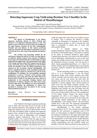
Figure 1: Example of Hants' algorithm for a pixel in sugarcane cultivation, applied on 10-day SPOT Vegetation images
Other two meteorological variables were Global
radiation and cumulative value for 10-day periods. Other
than latitude and longitude, the NDVI and MET data
were obtained from the current time frame starting from
2018 and running until 2020. To control for possible
cloud impacts. According to the researchers, Roerink et
al. (2000) briefly evaluates attributes such as the NDVI
temporal activity during the growing season as an up and
down in development. Because of that, the sequence was
changed by suppressing high frequency noise that was
deemed meaningless. The modification was based on a
minimal amount of quadric practical error. As an
example, take what would happen to a pixel's values if
there was a shift in sugarcane cultivation, and modify
them (up or down).
This research was conducted using a
Geographic Information System (GIS) to look at
sugarcane fields that are found only in sugarcane fields
in the areas of study. From the CANASAT (2007)
teratological map, an area map from maize, tobacco, and
sugar cane were drawn and planted coloured sugarcane
in the areas coloured it. Section 2 then, the NDVI time
series profiles were collected from each chosen pixel in
all territories and cropping seasons.
The average monitoring time series profile was
built and yielded now projections of the crop yields. By
averaging the noise profiles, the spectral data has been
scaled down to be sufficient in the qualitative details
required for the input. There is no reported daily weather
for each municipality. Instead, they use weekly averages
of meteorological readings from the national weather
service. A method for image data extraction was
rendered by using the ENVI computational system or the
IDL computational system based on the analysis carried
out by Esquerdo et al. in all of the 4 images (2006).The
defined technique of Lucas et al. relates to how plants
are classified as successful (Stable state, established)
during the vegetative development stage, then on the
next leg during the flowering / senesce stage, and finally
on the third leg during the formal harvest and extraction
(2005a). The accelerated development of the embryo
was split into two parts: quick growth and slow growth.
Thus, instead of having one key model, the development
adopted 4 separate phases: establishment, rapid growth,
slow growth, and stability / senesce.With 20
municipalities as the sample collection, the amount of
nitrogen is closely tracked from season to season, and a
median pattern from 20 seasons was analysed and
compared to determine the production of plant richness
for each cropping season. The phenological stages of
crop production were described in record vegetation
growth data, based on observations of a general activity
of NDVI data for seven years. After taking all the
readings, the NDVI measurements among each cropping

season are shown in the above image. Top row: average,
middle row: standard deviation, bottom row: sum of the
squares of standard deviation. Then, NDVI and
meteorological data were collated by phase, and the
spectra of light and the meteorological modelling were
conducted for each development phase, and the attributes
of light, wind, and temperature at each development
phase, emphasising that summer is the crop development
stage with the most spatially uniform attributes.
Table 1: Limits of classes for the average municipal yield and number of occurrences
Class Description Lower limit Upper limit Frequency
t ha-1
Low-medium 61 72 25 B-M
Medium 75 84 75 M
Medium-high 87 111 41 M-A
The accompanying graph illustrates how the
statistics tables demonstrate how these figures were
obtained as well as the lower and higher limits of the
sample sizes of these statistics and the number of
instances.A programme package called Weka was
employed to study the features collected and classified.
There were four techniques used for function selection:
After the above filtering process, Our goal was to
discover the kinds of attributes were chosen by the
plurality of approaches, which of those attributes were
the most important to decide the average regional yield
attribute.
To check the trend seen in the 2 ma correlation
study, two approaches were taken (a) using spectral
attributes and (b) using the average geographic yield.
The first method considered the average crop yield for
each season, considering the average crop yield in each
field. To measure the average spectral attribute (like
light, colour or sound) and the average crop yield among
the regions, one gathered all the data (the number of
crops planted in each location) for each particular area
and crop system. In order to analyse the average crop
yields annually, crops were analysed on a yearly basis,
not just a three year cycle. The average historical value
of spectral attributes and yields was determined with the
aid of all the municipalities.
IV. RESULT AND DISCUSSION
A table below the "Improvements" column
displays the chosen characteristics for each enhancement
process. The meteorological characteristics were chosen,
but by accident. It is likely that as a result of fixing the
development phases on the calendar for 2008, the
development phases for 2009, 2010 and 2021, as well as
the by implication of accumulated meteorological
results, were predetermined. The explanation that the
yield is not reported is due to the imprecise procedure for
discretization employed within this lab. In doing primary
analysis with percentiles system in place, the three
groups in percentiles did not catch the numeric choice
score well.
Table 2: Selected attributes for each attribute selection method
Attributes Phase Selection Methods
1 2 3 4
ndvi_1final 1 x
ndvi_1m 2 X X X
ndvi_2final 2 X X X
ndvi_3s 3 X X X
ndvi_3inic 3 X X X X
ndvim Whole crop X x X
ndvimax x
Decmax x x
Based on the above properties, the J48 category
program was implemented using a decision tree. The
cross validation approach was introduced by 5-folds, and
it had the consequence of successful prediction. In 140
applications, the classifier accurately predicted 70% of
the time, taking the error rate down to 40%. The
following table provides a summary of it.
Table 3: Confusion matrix and classification accuracy for yield rate from ndvi2_m, ndvi2_final, ndvi3_s, ndvi3_inic and
ndvi_m attributes
Classification/Original B-M M M-A Accuracy [%]
B-M 14.5 10 2.2 63%
M 6.4 54 12.5 74%
M-A 3 9 27 67%

It was found that there was a lack of balance
between the results, with more uncertainty occurring
between neighbouring classes than between distant
classes. It is possible that there is a misunderstanding
involved with the way that the attribute value class is
specified (average crop yield). The primary purpose of
the ndvi2 final and ndvi2 m features is to convert the
output of the tree level feature extraction stage to a
higher level feature-vector (NDVI2 VEC). These groups
are the fastest rising sub-sections of the group, gathered
during the growth process means that the area of crops
will be able to generate more high quality yields.
Then, a new classification was done by using
160 instances, which did not include the code "89" and
which contained 15 instances of the code "62". In order
to create a methodology to better distinguish the dataset,
the J48 classifier algorithm was used with ten items
required, and cross validation was used with five folds
for the training collection. If you had to score the
classifier on reviewing 66% of the cases, you could infer
that 94 out of 140 instances were correctly guessed.
Figure 2: Decision tree for yield classification using ndvi2_m, ndvi2_final, ndvi3_inic and ndvi_m attributes
Although there was a substantial deterioration
about the classification of yield BM, whose hit percent
decreased from 62.5 to 8.3. The study's results classified
M class yield increased from 74.3% to 86.5%. It's
accuracy percentage increased from 76% to 84%. So,
there is no improvement in the MA class'
recommendation for the application.
Table 4: Confusion matrix and classification accuracy for yield classification using ndvi2_m and ndvi2_final attributes
Classification/Original B-M M M-A Accuracy [%]
B-M 2 0 0 8%
M 20 65 15 85%
M-A 3 10 27 67%
In the above table, you can see that the average
municipality yield (as a percentage of raw input) was
calculated using only the ndvi2 m and ndvi2 final
attributes. Looking at all the master data descriptions
(ndvi2 m and ndvi2 final), it was determined that the
highest yields could be achieved with only the ndvi2 m
attributes, however), though both the ndvi2 m and ndvi2
final data were not able to demonstrate the plots that
were required. It is very critical that the conditions in the
field (field adaptation) must be optimal.

Figure 3: Decision tree for yield classification using ndvi2_final and ndvi2_m attributes
Correlation studies between both the two
spectral properties of phase 2 and the mean municipal
yield were performed to determine the trend seen in the
above graph, in which maximum value are linked to
organizational yield and vice versa. In the first solution
to the issue, the alternative under consideration was to
determine the average crop yield of a typical
municipality for the stated cropping season.
Figure 4: a) Correlation between ndvi final in phase 2 and average yield for each cropping season (considering different
regions). b) Correlation between average ndvi in phse 2 and average yield for each cop (considering different regions
The NDVI maps in the accompanying diagram
shows that the correlation findings between the
final/average NDVI, the NDVI from phase 2, and the
total return for each cropping season, considered
estimates among different area. Each capped circle in
graphs corresponds to one planting season. The findings
were consistent with the description provided in the
above diagram, i.e., cropping seasons with higher
spectral value of a dependent variable appeared to
produce higher yields and vice versa.
The goal of this approach was to check whether
the regional or seasonal yield historical trend (historical
sequence from 2013 to 2020) could be viewed in the
electronic spectrometer. The findings shown on the
following graph almost match the results of Image 10.
The low coefficient of determination may suggest these
effects were consistent, considering the low number of
patients who were involved in the study. The R2 value
for the results in Geouge was predicted to be lower than
that of other regions due to the impact of random
sampling on the results.

Figure 5: a) Correlation between final ndvi in phase 2 and average yield for each region - historical series between 2013 to
2020; b) Correlation between average ndvi in phase 2 and average yield for each region - historical series between 2013 to
2020
V. CONCLUSION
Despite being higher in accuracy than other
standards, they are good indicators for crop monitoring
purposes as used by the European Commission (JRC,
2010) as monthly crop bulletin monitoring basis, which
produces these bulletins based on NDVI signals, which
provide a basis for quantitative assessments of crop
growth. The FDA cites a study by CATHERINE
AGUSTIN, BA and BRENDA S.H. RANE in which
they note that there are various scientific studies on the
use of satellite imagery in farming, one of which is the
"Development of the Moderate Resolution Imaging
Spectroradiometer (MODIS) In Situ (MODIS-I) for Crop
Yield Estimation," which examining the ability of
satellite imagery to estimate crop yields for rice.
REFERENCES
[1] Boken, VK & Shayewich, CF. (2002). Improving an
operational wheat yield model using phenological phase-
based Normalized Difference Vegetation
Index. International Journal of Remote Sensing, 23,
4155-4168.
[2] Left, JCDM, Antunes, JFG; Baldwin, DG; Emery,
WJ, & Zullo Júnior, J. (2006). An automatic system for
AVHRR land surface product generation. International
Journal of Remote Sensing, 27, 3925-3942.
[3] Ferencz, C., Bognár, P., Lichtenberger, J., Hamar,
D., Tarcsai, G., Timár, G., Molnár, G., Pásztor,
S., Steinbach, P., Székely, B., Ferencz, OE, & Ferencz-
Árkos, I. (2004). Crop yield estimation by remote
sensing. International Journal of Remote Sensing, 25,
4113-4149.
[4] Greenland, D. (2005). Climate variability and
sugarcane yield in Louisiana. Journal of Applied
Meteorology, 44, 1655-1666.
[5] Fernandes et al. (2006). Joint Research Center
[JRC]. Meteorological data simulated by ECMWF
model. Available
at: http://mars.jrc.ec.europa.eu/mars/About-
us/FOODSEC/Data-Distribution.
[6] Joint Research Center [JRC]. (2006). Bulletins and
publications. Available
at: http://mars.jrc.ec.europa.eu/mars/Bulletins-
Publications.
[7] Labus, MP, Nielsen, GA, Lawrence, RL, & Engel, R.
(2002). Wheat yield estimates using multi-temporal
NDVI satellite imagery. International Journal of Remote
Sensing, 23, 4169-4180.
[8] Roerink, GJ, Menenti, M., & Verhoef, W. (2000).
Reconstructing cloudfree NDVI composites using
Fourier analysis of time series. International Journal of
Remote Sensing, 21, 1911-1917.
[9] Simões, MS, Rocha, JV, & Lamparelli, RAC.
(2005a). Spectral variables growth analysis and yield of
sugarcane. Scientia Agricola, 62, 199-207.
(2005b). Growth indices and productivity in
sugarcane. Scientia Agricola, 62, 23-30.
(2009). Orbital spectral variables, growth analysis and
sugarcane yield. Scientia Agricola, 66, 451-461.
[12] Ali MM, Qaseem MS, Rajamani L, & Govardhan
A. (2013). Extracting useful rules through improved
decision tree induction using information entropy. Int. J.
Inf. Sci. Techniques, 3(1), 27–41.
[13] Alparslan E, Coskun G, & Alganci U. (2009).
Water quality determination of Küçükçekmece lake,

Turkey by using multispectral satellite data. Sci. World
J., 9, 1215–1229.
[14] Anderson JR, Hardy EE, Roach JT, & Witmer RE.
(1976). A land use and land cover classification system
for use with remote sensor data. United States
Government Printing Office, Washington, DC.
[15] Avci ZU, Karaman M, Ozelkan E, & Papila I.
(2011). A comparison of pixel based and object-based
classification methods, a case study. Istanbul, Turkey.
[16] Avery TE & Berlin GL. (1992). Fundamentals of
remote sensing and airphoto interpretation. Prentice
Hall.
[17] Baret F & Guyot G. (1991). Potentials and limits of
vegetation indices for LAI and APAR assessment.
Remote Sens. Environ., 35, 161-173.
[18] Blackburn GA. (2007). Hyperspectral remote
sensing of plant pigments. J. Exp. Bot., 58, 855–867.
[19] Buschmann C & Nagel E. (1993). In vivo
spectroscopy and internal optics of leaves as basis for
remote sensing of vegetation. Int. J. Remote Sens., 14,
711–722.
[20] Chander G, Markham BL, & Helder DL. (2009).
Summary of current radiometric calibration coefficients
for Landsat MSS, TM, ETM+ and EO-1 ALI sensors.
Remote Sens. Environ., 113, 893–903.
[21] Congalton RG & Green K. (1999). Assessing the
accuracy of remotely sensed data: principles and
practices. Boca Raton: Lewis Publishers.
[22] Dai QY, Zhang CP, & Wu H. (2016). Research of
decision tree classification algorithm in data mining. Int.
J. Database Theory Appl., 9(5), 1–8.
[23] Deering DW. (1978). Rangeland reflectance
characteristics measured by aircraft and spacecraft
sensors. Ph.D Dissertation. Texas A & M University,
College Station, pp. 338.
[24] Deering DW, Rouse JWJ, Haas RH, & Schell JA.
(1975). Measuring forage production of grazing units
from Landsat MSS data. In: 10th International
symposium on Remote Sensing of Environment, pp.
1169–1179.
[25] De Fries RS, Hansen M, Townshend JR, &
Sohlberg R. (1998). Global land cover classifications at
8 km spatial resolution: the use of training data derived
from Landsat imagery in decision tree classifiers. Int. J.
Remote Sens., 19(16), 3141–3168.

Detecting Sugarcane Crop Yield using Decision Tree Classifier in the District of Muzaffarnagar

Recommended

Recommended

More Related Content

Similar to Detecting Sugarcane Crop Yield using Decision Tree Classifier in the District of Muzaffarnagar

Similar to Detecting Sugarcane Crop Yield using Decision Tree Classifier in the District of Muzaffarnagar (20)

More from Dr. Amarjeet Singh

More from Dr. Amarjeet Singh (20)

Recently uploaded

Recently uploaded (20)

Detecting Sugarcane Crop Yield using Decision Tree Classifier in the District of Muzaffarnagar