Download to read offline


![Bucket Sort
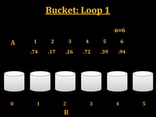
Bucket sort assumes that the input is generated by a random
process and drawn from a uniform distribution.
In other words the elements are distributed uniformly and
independently over the interval [0,1].
Bucket sort divides the interval [0,1] into n equal sized
subintervals or buckets. Then distributes the n inputs into
these buckets.
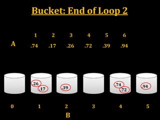
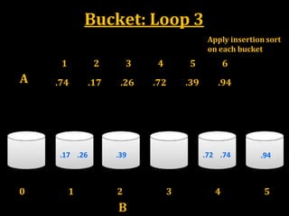
After that the elements of each buckets are sorted using a
sorting algorithm generally using insertion or quick sort.
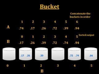
Finally the buckets are concatenated together in order.
Consider that the input is an n-element array A and each
element A[i] in the array satisfies the 0<=A[i]<1](https://image.slidesharecdn.com/adalinearsorting-190310082711/85/Linear-Sorting-6-320.jpg)
![Bucket Sort Algorithm
Bucket-Sort(A)
1. Let B[0….n-1] be a new array
2. n = length[A]
3. for i = 0 to n-1
4. make B[i] an empty list
5. for i = 1 to n
6. do insert A[i] into list B[ n A[i] ]
7. for i = 0 to n-1
8. do sort list B[i] with Insertion-Sort
9. Concatenate lists B[0], B[1],…,B[n-1] together in
order](https://image.slidesharecdn.com/adalinearsorting-190310082711/85/Linear-Sorting-7-320.jpg)
![Bucket: Loop 2
A
2 3 4 5 6
.17 .26 .72 .39 .94
B[ n A[i] ] = B[ 6X.74 ]=B[ 4.44 ]=B[4]
0 1 2
B
3 4 5
FOR n=6, i=1
1
.74](https://image.slidesharecdn.com/adalinearsorting-190310082711/85/Linear-Sorting-10-320.jpg)
![Bucket: Loop 2
A
1
.74
3 4 5 6
.26 .72 .39 .94
B[ n A[i] ] = B[ 6X.17 ]=B[ 1.02 ]=B[1]
FOR n=6, i=2
.74
2
.17
0 1 2
B
3 4 5](https://image.slidesharecdn.com/adalinearsorting-190310082711/85/Linear-Sorting-11-320.jpg)
![Bucket: Loop 2
A
1 2
.74 .17
4 5 6
.72 .39 .94
B[ n A[i] ] = B[ 6X.26 ]=B[ 1.56 ]=B[1]
FOR n=6, i=3
.74
3
.26
.17
0 1 2
B
3 4 5](https://image.slidesharecdn.com/adalinearsorting-190310082711/85/Linear-Sorting-12-320.jpg)
![Bucket: Loop 2
A
1 2 3
.74 .17 .26
5 6
.39 .94
B[ n A[i] ] = B[ 6X.72 ]=B[ 4.32 ]=B[4]
FOR n=6, i=4
.74
4
.72
.26
.17
0 1 2
B
3 4 5](https://image.slidesharecdn.com/adalinearsorting-190310082711/85/Linear-Sorting-13-320.jpg)
![Bucket: Loop 2
A
1 2 3 4
.74 .17 .26 .72
6
.94
B[ n A[i] ] = B[ 6X.39 ]=B[ 2.34 ]=B[2]
FOR n=6, i=5
5
.39
.17
.26 .74
.72
0 1 2
B
3 4 5](https://image.slidesharecdn.com/adalinearsorting-190310082711/85/Linear-Sorting-14-320.jpg)
![Bucket: Loop 2
A
1 2 3 4 5
.74 .17 .26 .72 .39
B[ n A[i] ] = B[ 6X.94 ]=B[ 5.64 ]=B[5]
FOR n=6, i=6
6
.94
.17
.26 .74
.72.39
0 1 2
B
3 4 5](https://image.slidesharecdn.com/adalinearsorting-190310082711/85/Linear-Sorting-15-320.jpg)
![Analysis of Bucket Sort
1. Let B[0….n-1] be a new array
2. n = length[A]
3. for i = 0 to n-1
4. make B[i] an empty list
5. for i = 1 to n
6. do insert A[i] into list B[ floor of n A[i] ]
7. for i = 0 to n-1
Bucket-Sort(A)
8. do sort list B[i] with Insertion-Sort
9. Concatenate lists B[0], B[1],…,B[n-1] together in
order
Step 5 and 6
takes O(n)
time
Step 7 and 8
takes O(n
log(n/k) time
Step 9 takes
O(k) time
In total Bucket sort takes : O(n) (if k=Θ(n))](https://image.slidesharecdn.com/adalinearsorting-190310082711/85/Linear-Sorting-19-320.jpg)
![Counting sort
Counting sort assumes that each of the n input elements is an
integer in the range 0 to k. that is n is the number of elements and
k is the highest value element.
Consider the input set : 4, 1, 3, 4, 3. Then n=5 and k=4
Counting sort determines for each input element x, the number of
elements less than x. And it uses this information to place
element x directly into its position in the output array. For
example if there exits 17 elements less that x then x is placed into
the 18th position into the output array.
The algorithm uses three array:
Input Array: A[1..n] store input data where A[j] {1, 2, 3, …, k}
Output Array: B[1..n] finally store the sorted data
Temporary Array: C[1..k] store data temporarily](https://image.slidesharecdn.com/adalinearsorting-190310082711/85/Linear-Sorting-21-320.jpg)
![Counting Sort
1. Counting-Sort(A, B, k)
2. Let C[0…..k] be a new array
3. for i=0 to k
4. C[i]= 0;
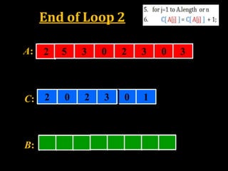
5. for j=1 to A.length or n
6. C[ A[j] ] = C[ A[j] ] + 1;
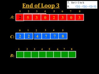
7. for i=1 to k
8. C[i] = C[i] + C[i-1];
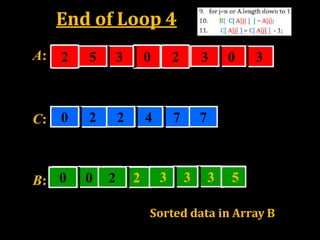
9. for j=n or A.length down to 1
10. B[ C[ A[j] ] ] = A[j];
11. C[ A[j] ] = C[ A[j] ] - 1;](https://image.slidesharecdn.com/adalinearsorting-190310082711/85/Linear-Sorting-22-320.jpg)
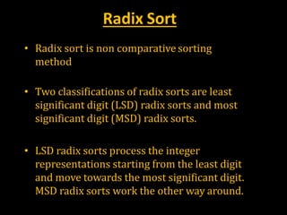
![Time Complexity Analysis
[Loop 1]
[Loop 2]
[Loop 3]
[Loop 4]
1. Counting-Sort(A, B, k)
2. Let C[0…..k] be a new array
3.for i=0 to k
4. C[i]= 0;
5. for j=1 to A.length or n
6. C[ A[j] ] = C[ A[j] ] + 1;
7. for i=1 to k
8. C[i] = C[i] + C[i-1];
9. for j=n or A.length down to 1
10. B[ C[ A[j] ] ] = A[j];
11. C[ A[j] ] = C[ A[j] ] - 1;
Loop 2 and 4
takes O(n) time
Loop 1 and 3
takes O(k) time](https://image.slidesharecdn.com/adalinearsorting-190310082711/85/Linear-Sorting-29-320.jpg)


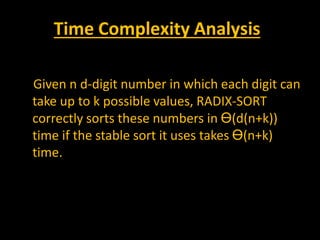
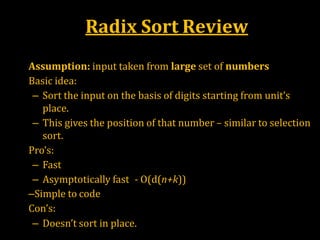
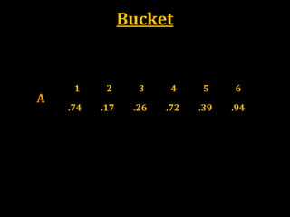
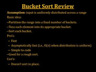
The document provides an analysis and design of algorithms focusing on linear time sorting methods, specifically bucket sort, radix sort, and counting sort. It describes the mechanisms, time complexities, pros, and cons of each sorting algorithm. Each method is evaluated based on its assumptions, implementation steps, and performance considerations.