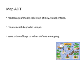
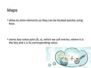
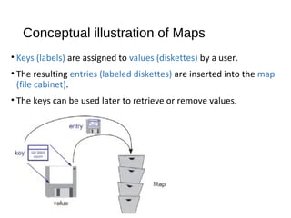
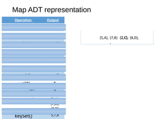
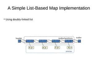
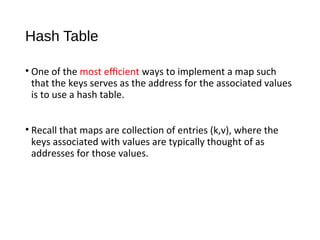
The document describes maps and hash tables as data structures that store unique key-value entries for efficient retrieval. It details methods for map operations like adding, retrieving, and removing entries, along with the concept of hash tables that use a bucket array and hashing functions for faster access. Various collision resolution techniques, such as separate chaining and open addressing, are also covered, highlighting their implementation strategies and time complexities.

1. Maps & Hash Tables

2. Map ADT
• models a searchable collection of (key, value) entries.
• requires each key to be unique.
• association of keys to values defines a mapping.

3. Maps
• allow to store elements so they can be located quickly using
keys.
• stores key-value pairs (k, v), which we call entries, where k is
the key and v is its corresponding value.

4. Conceptual illustration of Maps
• Keys (labels) are assigned to values (diskettes) by a user.
• The resulting entries (labeled diskettes) are inserted into the map
(file cabinet).
• The keys can be used later to retrieve or remove values.

5. Applications
• address book.
• student-record database.

6. Map ADT methods
• size():
• Deterines the size of Map M.
• isEmpty():
• Test whether M is empty.
• get(k):
• If M contains an entry e=(k,v), where k is key, then return the value v, else
return null.

7. Map ADT methods
• put(k,v):
• If M does not have an entry (k,v) , then add entry (k,v) to M and
return null; else, replace with v the existing value of the entry with “k”
key and return the old value.
• remove(k):
• Remove from M the entry with key equal to k, and return its value.
•keySet():
• Return an iterable collection containing all the keys stored in M.

8. Map ADT methods
• values():
• Return an iterable collection containing all the values associated with keys
stored in M.
• entrySet():
• Return an iterable collection containing all the key-value entries in M.

9. Map ADT representation
Operation Output
put(5,A) null
put(7,B) null
put(2,C) null
put(8,D) null
put(2,E) C
get(7) B
get(4) null
get(2) E
remove(2) E
entrySet() (5,A),
(7,B),
(8,D)
keySet() 5,7,8
(7,B)
,
(5,A), (2,C), (8,D),(2,E),

10. A Simple List-Based Map Implementation
• Using doubly-linked list

11. Performance of a List-Based Map
In unsorted list
• Put(k,v)  O(1) time
• Get(k), remove(key)  O(n) time.

12. Hash Table
• One of the most efficient ways to implement a map such
that the keys serves as the address for the associated values
is to use a hash table.
• Recall that maps are collection of entries (k,v), where the
keys associated with values are typically thought of as
addresses for those values.

13. Hash Table components
• In general, a hash table consists of two major components, a
bucket array and a hash function.
• A bucket array
• A hash function.

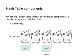
14. Bucket Array
• Consider array A of size N (array size)
• each cell is a bucket (i.e. a collection of (k,v))
• The keys of entries are integers in the range of [0, N-1], each
bucket holds at most one entry.
• Search, insertion and removal in the bucket array seems to take
O(1) time.

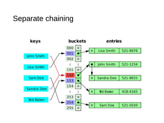
15. Bucket Array(cont.)
• It has two drawbacks:
• As the space used is proportional to N (array size).
• if N >> number of entries n present in the map, there is a waste of space.
• keys are required to be integers (range [0, N − 1]), which is often not the case.
• Overcome:
• Use the bucket array in conjunction with a "good" mapping from the keys to the
integers in the range [0,N − 1] like hash functions.

16. Hash functions (h)
• Is second part of hash table structure.
• Hash function value, h(k), is an index into the bucket array,
instead of k.
• So entry (k, v) is stored in the bucket A[h(k)].

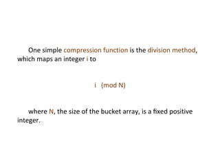
17. Evaluation of a hash function, h(k),
• Consists of two functions:
• mapping the key k to an integer, called the hash code.
• mapping the hash code to an integer within the range of
indices ([0, N − 1]) of a bucket array, called the
compression function.
• Hash codes may be generated by casting to an integer,
summing components, Polynomial hash codes etc.

18. One simple compression function is the division method,
which maps an integer i to
i (mod N)
where N, the size of the bucket array, is a fixed positive
integer.

19. Collision Handling Schemes
Collision occurs when different elements are mapped to the same cell.
Some collision resolution methods:
• Separate Chaining
• Open Addressing

20. Separate chaining

21. Separate chaining
• To index the n entries of map in a bucket array of capacity N.
• Each bucket has to be of size n/N called as the load factor of
the hash table.
• So the expected running time of operations is O(n/N).
• These operations can be implemented to run in O(1) time,
provided n is O(N).

22. Open Addressing

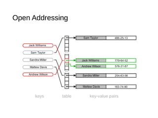
23. Linear probing
• Distance between probes is constant (i.e. 1, when probe
examines consequent slots).
• When an entry into a bucket A[i] is already occupied,
where i = h(k) then :
• Try next at A[(i + 1) modN]. If this is also occupied, then
• Try A[(i + 2) mod N], and so on.
• until we find an empty bucket that can accept the new entry.

24. Open Addressing with Linear Probing Strategy
Insert keys 18, 41, 22, 44, 59, 32, 31, 73 in this order to a bucket, using
h(k) = k (mod 13).
41 18 44 59 32 22 31 73
0 1 2 3 4 5 6 7 8 9 10 11 12

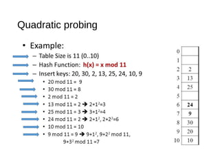
25. Quadratic probing
• trying the buckets
A[h(k) + j2] (mod N), for j = 0,1,..., N −1
until finding an empty bucket.
• N has to be a prime number.
• Bucket array must be less than half full.

26. Quadratic probing

27. Double Hashing
• Handles collision , by placing an item in the series:
H(k) = (h(k) + j × h’(k)) mod N for j = 0,1,...N −1.
• h’(k) cannot have zero values.
• Table size N must be a prime number.
• Common choice of compression function :
h’(k) = q – (k mod q) where q < N is a prime.

28. Open Addressing with Double Hashing Strategy
Insert keys 18, 41, 22, 44, 59, 32, 31, 73 in this order to a
bucket, using double-hashing resolution where:
h(k) = k (mod 13) and h’(k) = 7 – k (mode 7).
41 18 445932 2231 73
0 1 2 3 4 5 6 7 8 9 10 11 12
H(k) = (h(k) + j × h’(k))
= 5 + 1 x (7 – 44%7)
= 10
H(k) = (h(k) + j × h’(k))
= 5 + 1 x (7 – 31%7)
= 9
H(k) = (h(k) + j × h’(k))
= 5 + 2 x (7 – 31%7)
= 13

29. • Worst-case for insertions, removal, and searches, on a hash
table take O(n) time.
• The worst-case  all the keys inserted into the map collide.
• The load factor α = n/N affects the performance of hash
table.

30. Ordered Maps
• To keep the entries in a map sorted according to some order
• To look up keys and values based on this ordering.
• Performs the usual map operations, maintaining an order relation
for the keys.
• The worst-case time for searching in hash tables is O(n).
• A list implementation of an ordered array (known as ordered search
table), has O(lgn) as the worst-case time for searching.

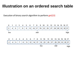
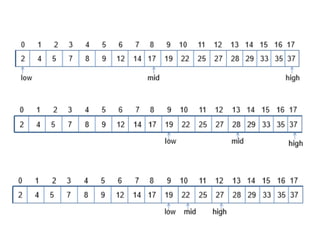
31. Searching algorithm – Binary search
Algorithm BinarySearch(S, k, low, high)
if low > high then
return null
else
mid ← [(low + high)/2 ]
e ← S.get(mid)
if k = e.getKey() then
return e
else if k < e.getKey() then
return BinarySearch(S, k, low, mid-1)
else
return BinarySearch(S, k, mid+1, high)

32. Illustration on an ordered search table
Execution of binary search algorithm to perform get(22)