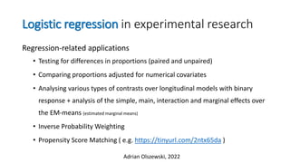
1. Logistic regression in experimental research
Regression-related applications
• Testing for differences in proportions (paired and unpaired)
• Comparing proportions adjusted for numerical covariates
• Analysing various types of contrasts over longitudinal models with binary
response + analysis of the simple, main, interaction and marginal effects over
the EM-means (estimated marginal means)
• Inverse Probability Weighting
• Propensity Score Matching ( e.g. https://tinyurl.com/2ntx65da )
Adrian Olszewski, 2022

2. Logistic regression – a few facts. 1/2
• A regression model for categorical endpoints / responses (here: binary) used to analyze the impact
(magnitude, direction, inference) of predictor variables on the probability of occuring an event.
• As every regression, it predicts a numerical outcome: E(Y|X=x). For the Bernoulli’s distribution (or
binomial with k=1) it’s a probability of success (or log-odds, dependeing on formulation). More
precisely, it’s a direct probability estimator.
• Logistic regression itself does NOT produce labels. More precisely, it’s a direct probability estimator. To
give classes, it needs additional post-fit activity: applying a decision rule to the predicted probability.
This makes the logistic classifier, which is a 3-step procedure:
1) Train the logistic regression model on existing data to to get the model coefficients
2) Predict the probability using a new data and the obtained model coefficients
3) Apply the decision rule to the probability to obtain the class
I hope everyone can see with own eyes that logistic classifier ≠ a logistic regression (it uses the LR)
• The ML community uses it entirely for classification. But, instead of using a proper name: „logistic
classifier”, they took over the name and completely replaced meanings. Today they claim that „logistic
regression is not a regression”, denying what thousands of people do at work every day. In my work, the
LR is not used for classification.

3. Logistic regression – a few facts. 2/2
• LR is fit by the Maximum Likelihood (it’s NOT just OLS with logit transformation)
https://stats.stackexchange.com/questions/48485/what-is-the-difference-between-logit-transformed-linear...
• LR is part of the Generalized Linear Model (like linear, Poisson, gamma, beta, etc.). Technically there’s no
difference for the fitting algorithm which one you choose. Just specify the binomial conditional distribution
and logit link (or probit – for a less convenient interpretation) and get the table of model coefficients.
• LR was invented in 1958 by sir Cox (traces of the logistic function reach the 19th century:
https://papers.tinbergen.nl/02119.pdf ; Verhulst, Quetelet, Pearl) and multinomial LR in 1966. It was then
generalized by Nelder and Wedderburn into a general GLM framework. Hastie and Tibshirani invented then
the GAM (Generalized Additive Model) allowing for non-linear predictor.
Hastie authored the glm() command in the S-PLUS statistical suite (the father of R, origin of the R syntax),
estimating the coefficients of the regression models and performing the inference. Additional extensions for
handling repeated observations were made by Liang and Zieger in 1986 (GEE – Generalized Estimating
Equations) and Breslow, Clayton and others around 1993 (GLMM – generalized linear mixed models).
• https://www.jmp.com/content/dam/jmp/documents/en/statistically-speaking-resources/statspkg-stroup-
glmms.pdf

4. Logistic regression – a few facts. 2/2

5. LR can replace the classic statistical tests for comparison of % of success*:
(but not % being any ratio  then use beta regression, simplex regression, fractional logistic regression, GEE estimated linear model)
- 2/n-sample between independent groups (ordinary)
- 2/n-sample between dependent groups (via GEE estimation or a mixed model)
- Over time – (linear, quadratic, cubic) trend in % (via GEE estimation or a mixed model)
• to compare percentage structures over 2+ categories the multinomal logistic regression is used
• If the compared classes are ordered, the proportional-odds model can be used (aka ordinal LR)
• If the proportionality of odds doesn’t hold, the Generalized Ordinal LR can be employed
• If the compared classes are dependend (nested), the hierarchical multinomial LR is used
• BTW: the Ordinal Logistic Regression is a generalization of the Wilcoxon (Mann-Whitney) test.
https://www.fharrell.com/post/powilcoxon/ | https://www.fharrell.com/post/rpo/

6. LR allows one to analyze longitudinal studies with binary endpoint (observations repeated over time)
- assessment of specific contrasts (simple effects): Tukey (all-pairwise), Dunnett (all-vs. control), selected, trends.
- n-way comparisons across many categorical variables & their interactions.
- the comparisons can be adjusted for numerical covariates.
- followed by the LRT or Wald’s testing  AN(C)OVA („analysis of deviance”) for the main & interaction effects.
- marginal effects express the predictions in „percentage-points” rather than „odds ratios” or „probabilities”.
- allows for using time-varying covariates and piecewise analysis.
- GEE estimation allows for population-average comparisons.
Mixed-effect model allows for comparisons conditional on subject.
The two answer different questions and cannot be used interchangeably.
- In presence of missing data, the Inverse Probability Weighting can be employed
to prevent biased estimates. The IPW also uses the LR internally 
- Both using smoothing terms (splines) or employing the the GAM approach
(invented by Hastie & Tibshirani) can handle non-linearity in the predictor.
- LASSO or Ridge regularization can be used in case of multi-collinearity.
A1
B
C
A1:B
1

7. Study arm 1 Baseline numerical
covariates to adjust for
2% 15% 30% 60% 78%
Study arm 2 0% 12% 18% 20% 45%
Time Baseline (T0) T1 T2 T3 T4 ….
Pre-treatment Post-treatment
• All-pairwise comparisons (rather exploratory, not much useful if not supported by some clinical justification):
• Arm1-T1 vs. Arm1-T2
• Arm1-T1 vs. Arm1-…
• Arm1-T1 vs. Arm2-T1
• Arm1-T1 vs. Arm2-T2, …
• Between-treatment comparison (typical analysis in clinical trials; particular focus on selected timepoint(s)  primary objective)
• T1-Arm1 vs. T1-Arm2
• T2-Arm1 vs. T2-Arm2
• T3-Arm1 vs. T3-Arm2, …
• Within-treatment comparison (sometimes practiced, but much criticized as not a valid measure of clinical effect)
• Arm1: T1 vs. T2, T1 vs. T3, T1 vs. T…, T2 vs. T3, T2 vs. T…
• Arm2: T1 vs. T2, T1 vs. T3, T1 vs. T…, T2 vs. T3, T2 vs. T…
• Comparison of difference in trends (sometimes practiced, must be supported by valid clinical reasoning)
• Arm1 – Linear (Quadratic, …) vs. Arm2 – Linear (Quadratic, …)
Analyses of contrasts over a longitudinal model with a binary endpoint (SUCCESS/FAILURE)

8. Term Estimate SE p-value
Treatment xxx xxx p=0.0032
Time xxx xxx p=0.0001
Site xxx xxx p=0.98
Numerical_covar_1 xxx xxx p=0.101
Treatment*Time xxx xxx p=0.004
Treatment*Site xxx xxx p=0.87
….
Analyses of deviance [Type-2 or Type-3 AN(C)OVA]
Success ~ Treatment * Time * Site * Numerical_covariate1 + Baseline_covariate_1 + …..
Analyses of interactions over the EM-means*
(*estimated marginal means = LS-means)
T1 T2 T3 T4 T5 0 0.1 0.2 0.3 0.4 0.5 0.6 0.7 0.8 0.9
Comparing (nested) models – one per model term – via
sequence of Likelihood Ratio Tests (LRT)
Using Wald’s joint testing over appropriate model coefficients
(Wald is less precise but faster and always available)

9. There are so many members of the Logistic Regression family!
✅ Binary Logistic Regression = binomial regression with logit link, case of the Generalized Linear Model, modelling the % of successes.
✅ Multinomial Logistic Regression (MLR) = if we deal with a response consisting of multiple non-ordered classes (e.g. colours).
✅ Nested MLR - when the classes in MLR are related
✅ Ordinal LR (aka Proportional Odds Model) = if we deal with multiple ordered classes, like responses in questionnaires, called Likert
items, e.g. {bad, average, good}. The OLR is a generalization of the Mann-Whitney (-Wilcoxon) test, if you need a flexible non-parametric
test, that: a) handles multiple categorical variables, b) adjusts for numerical covariates (like ANCOVA)
✅ Generalized OLR = Partial Proportional Odds M. when the proportionality of odds doesn't hold.
✅ Alternating Logistic Regression = if we deal with correlated observations, e.g. when we analyse repeated or clustered data. We have
3 alternatives: mixed-effect LR, LR fit via GEE (generalized estimating equations), or alternatively, the ALR. ALR models the dependency
between pairs of observations by using log odds ratios instead of correlations (like GEE). It handles ordinal responses.
✅ Fractional LR = if we deal with a bounded range. Typically used with [0-100] percentages rather than just [TRUE] and [FALSE]. More
flexible than beta reg., but not as powerful as the simplex reg. or 0-1-inflated beta r.
✅ Logistic Quantile Regression - application as above.
✅ Conditional LR = if we deal with stratification and matching groups of data, e.g. in observational studies without randomization, to
match subjects by some characteristics and create homogenous "baseline".

10. A few books about the logistic regression (and the entire GLM) in experimental research

11. Testing hypotheses about binary outcomes (proportions)
with the Logistic Regression & selected friends
Logistic Regression
Ordinal
Logistic Regression
Logistic Regression
via GEE & GLMM
Conditional
Logistic Regression
Adrian Olszewski (2023)
In general for
paired / dependent data
Paired testing via GEE

12. > # =================| (Cochrane-) Mantel-Haenszel |=================
> tidy(mantelhaen.test(data$response, data$trt, data$gender, exact = F, correct = F))
estimate statistic p.value parameter conf.low conf.high method alternative
1 3.31 8.31 0.00395 1 1.45 7.59 Mantel-Haenszel chi-squared test without continuity correction two.sided
> summary(clogit(response~trt + strata(gender), data=data))$sctest
test df pvalue
8.305169 1.000000 0.003953
> # =================| Breslow-Day |=================
> tidy(BreslowDayTest(xtabs(~ trt +response + gender, data=data), correct = TRUE))
statistic p.value parameter method
1 1.49 0.222 1 Breslow-Day Test on Homogeneity of Odds Ratios (with Tarone correction)
> as.data.frame(anova(glm(response ~ trt * gender , data = data, family = binomial(link = "logit")), test="Rao")[4, ])
Df Deviance Resid. Df Resid. Dev Rao Pr(>Chi)
trt:gender 1 1.499 102 130.1 1.497 0.2212
> # =================| Rao z test |=================
> tidy(prop.test(xtabs(~ trt + response, data=data), correct = FALSE))
estimate1 estimate2 statistic p.value parameter conf.low conf.high method alternative
1 0.509 0.235 8.44 0.00366 1 0.0977 0.450 2-sample test for equality of proportions without … two.sided
> broom::tidy(chisq.test(xtabs(~ trt + response, data=ddata), correct = FALSE))
statistic p.value parameter method
1 8.44 0.00366 1 Pearson's Chi-squared test
> as.data.frame(anova(glm(response ~ trt , data = data, family = binomial(link = "logit")), test = "Rao"))[2, ]
Df Deviance Resid. Df Resid. Dev Rao Pr(>Chi)
trt 1 8.626 104 131.9 8.443 0.003665
> # =================| Wald's z test |=================
> margins::margins_summary(glm(response ~ trt , data = data, family = binomial(link = "logit")))
factor AME SE z p lower upper
trtplacebo 0.2738 0.0898 3.0475 0.0023 0.0977 0.4499
> marginaleffects::avg_slopes(glm(response ~ trt , data = data, family = binomial(link = "logit")))
Term Contrast Estimate Std. Error z Pr(>|z|) S 2.5 % 97.5 %
trt placebo - active 0.274 0.0898 3.05 0.00231 8.8 0.0977 0.45
Columns: term, contrast, estimate, std.error, statistic, p.value, s.value, conf.low, conf.high
> pairs(emmeans(glm(response ~ trt , data = data, family = binomial(link = "logit")), regrid="response", specs = ~ trt))
contrast estimate SE df z.ratio p.value
active - placebo -0.274 0.0898 Inf -3.047 0.0023
> wald_z_test(xtabs(~ trt + response, data=data))
z se p.value
1 3.047 0.08984 0.002308
wald_z_test <- function(table) {
p1 <- prop.table(table, 1)[1,1]
p2 <- prop.table(table, 1)[2,1]
n1 <- rowSums(table)[1]
n2 <- rowSums(table)[2]
se_p1 <- sqrt(p1 * (1 - p1) / n1)
se_p2 <- sqrt(p2 * (1 - p2) / n2)
se_diff <- sqrt(se_p1^2 + se_p2^2)
z <- (p1 - p2) / se_diff
p <- 2 * (1 - pnorm(abs(z)))
return(data.frame(z = z, se = se_diff,
p.value = p, row.names = NULL))
}

13. > # =================| McNemar's test |=================
> tidy(mcnemar.test(x=paired_data[paired_data$Time == "Pre", "Response"], y=paired_data[paired_data$Time == "Post", "Response"], correct = F))
statistic p.value parameter method
1 10.3 0.00134 1 McNemar's Chi-squared test
> paired_data %>% rstatix::friedman_test(Response ~ Time |ID)
.y. n statistic df p method
1 Response 20 10.3 1 0.00134 Friedman test
> RVAideMemoire::cochran.qtest(Response ~ Time | ID, data=paired_data)
Cochran's Q test
data: Response by Time, block = ID
Q = 10.29, df = 1, p-value = 0.001341
alternative hypothesis: true difference in probabilities is not equal to 0
sample estimates:
proba in group Post proba in group Pre
0.7 0.1
> coef(summary(geepack::geeglm(Response ~ Time, id = ID, data=paired_data, family = binomial(), corstr = "exchangeable")))[2,]
Estimate Std.err Wald Pr(>|W|)
TimePre -3.045 0.9484 10.31 0.001327
> # =================| Cochrane-Armitage s test |=================
> # (approximate!)
> tidy(DescTools::CochranArmitageTest(xtabs(~Response + Time, data=trend)))
statistic p.value parameter method alternative
1 -3.59 0.000336 3 Cochran-Armitage test for trend two.sided
> rstatix::prop_trend_test(xtabs(~Response + Time, data=trend))
n statistic p p.signif df method
1 30 12.9 0.000336 *** 1 Chi-square trend test
> as.data.frame(anova(glm(Response ~ Time, data=trend, family = binomial()), test="LRT"))[2,]
Df Deviance Resid. Df Resid. Dev Pr(>Chi)
Time 2 14.99 27 26.46 0.0005553
> joint_tests(emmeans(glm(Response ~ Time, data=trend, family = binomial()), specs = ~Time, regrid="response"))
model term df1 df2 F.ratio p.value
Time 2 Inf 17.956 <.0001

14. Sad reality in data science and machine learning… People have started to deny the reality…

15. Sad reality in data science and machine learning… People have started to deny the reality…