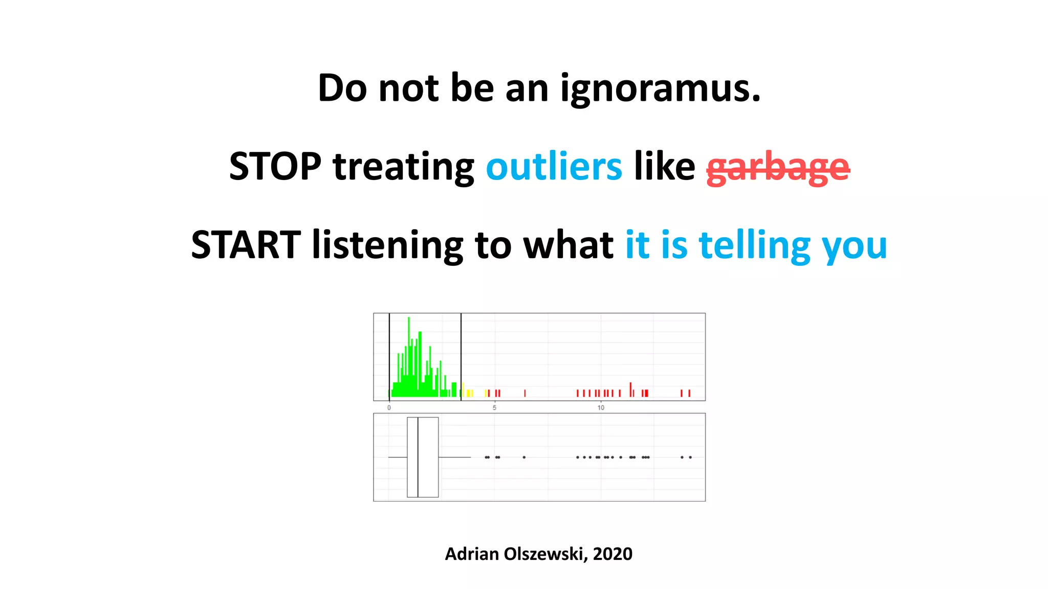
The document emphasizes the importance of not disregarding outliers in data analysis, warning that outliers may indicate data collection errors or signal critical issues, as demonstrated by the Flint water crisis. It critiques common statistical methods for outlier detection that lack context and cautions against blindly removing outliers, as they can represent meaningful deviations rather than errors. The author advocates for careful examination of outliers in conjunction with clinical and contextual understanding to avoid misinterpretation of the data.

1. Do not be an ignoramus.
STOP treating outliers like garbage
START listening to what it is telling you
Adrian Olszewski, 2020

2. 1. Outliers being confirmed errors may indicate problems with the data acquisition process:
a) Procedural issues
b) poor data entry validation mechanisms, allowing incorrect data to pass to the database
2. A few confirmed non-error outliers may warn, that something very bad is about to happen, like in the Flint Water Crisis, where
people got poisoned with lead, due to ignored (excluded) outliers
Read it and think twice, before you follow „data science guru” saying about „automated removal of outliers”
a) Langkjær‐Bain, R. (2017), The murky tale of Flint's deceptive water data. Significance, 14: 16-21. doi:10.1111/j.1740-9713.2017.01016.x,
https://rss.onlinelibrary.wiley.com/doi/full/10.1111/j.1740-9713.2017.01016.x
“There are a lot of statistical methods looking at whether an outlier should be deleted,” says Barry Nussbaum, the president of the American
Statistical Association. “I don't endorse any of them.” Nussbaum knows plenty about environmental statistics – he served as chief statistician
at the EPA until early last year (although he was not involved with the Flint case). He says: “Typically you do omit outliers if there is some
measurement problem among the very high or low observations. But if it is a properly measured value, you must investigate further. You must
look at those outliers and ask, what's going on here? To just delete it because it's an outlier is completely wrong.”
b) Wicklin R (2017), 5 Statistical Lessons from the Flint Water Crisis, https://www.linkedin.com/pulse/5-statistical-lessons-from-flint-water-crisis...
What do outliers may tell us?

3. 3. Numerous non-error outliers often indicate mixed samples from 2+ populations. It happens, if we fail at defining our model, e.g. miss
a covariate, that could separate them into own groups or assume wrong distribution
• I wish you luck with with applying methods expecting the normal distribution to Poisson, gamma or – especially – log-normal.
Expect negative age (see my topic on LinkedIn) or a situation, when range: mean + 16xSD covers valid results (see on LinkedIn).
3. Often, especially in biosciences, we work with data, which (large) skewness is an immanent property of. It happens when
a) the data are counts
b) the data come from a process that „enforces” skewness. Good example is a clinical trial, in which only severely ill patients are
eligible to enter the study, which is driven by appropriate inclusion and exclusion criteria. As they recover, over time, we obtain
a mixture of high values (from ill or non-responding patients) and low values (from recovering ones)
c) the data come from a process of multiplicative nature
d) The data are naturally truncated and skewed, like concentrations. In biosciences it is not uncommon to have valid data of
3 orders of magnitude in a single data set. If I wanted to remove all outliers from my clinical datasets, I would need to halve
them and throw away the most important half…
What do outliers may tell us?

4. Most of the statistical methods of detecting outliers you are likely to learn (MOOC, universities, YouTube, blogs):
1. Ignore the context. It’s just a mathematical formula, which doesn’t „think” and „has no idea” about the origin of your data and what
it actually means. It calculates some metrics and compares the outcome to some threshold. That’s it.
Context comes from the circumstances and the knowledge about the researched phenomenon. Without it – you juggle numbers.
2. Give you false impression that everything is OK only because it didn’t find anything. Remember, the worst may not be visible.
3. May tempt you to remove (exclude) the outliers. Iteratively. If you remove one, the distribution changes. You may find another one.
And another. And another. Untill you data gets „castrated” and starts resembling the normal distribution.
4. Some of the methods assume additive nature of data, so they expect the normal distribution (e.g. Grubbs, 3xSD). If you use these
methods to data naturally (and strongly) skewed, prepare for nonsenses. Especially with the log-normal.
5. Single-dimensional methods may not be able to detect multi-dimensional outliers. Never forget that, if you work with complex data!
https://stats.stackexchange.com/questions/213/what-is-the-best-way-to-identify-outliers-in-multivariate-data
Details matter

5. A few words of explanation before we start…
• SDV – source data verification: verification of the data entered to a database against the source (e.g. paper) documentation
• MDV – medical data review: verification of the data (any) against the domain (here: clinical) relevance by a domain specialist (physician)
• Late (post-factum) validation – a validation done during the systematic data review or even the analysis („strange, that looks weird…”)
• Inclusion / Exclusion criteria – as set of rules determining whether a patient is eligible to enter the trial
• Reference Range [RR] – a range covering values of a certain clinical parameter deemed as normal in a population of healthy patients
• Observation out of the RR (o.o. RR) and clinically non-significant – a value of a certain clinical parameter, which exceeds the RR, but
is treated by the physician as normal (not worrying) given the circumstances.
For example, the physician knows that patient ate something sweet or greasy, drunk water, did gymnastics shortly before the blood test).
Examples: glucose 105mg/dL, AspAT 45 IU/L (or even 110 IU/L, if you ate pizza and drunk alcohol a few hours earlier)
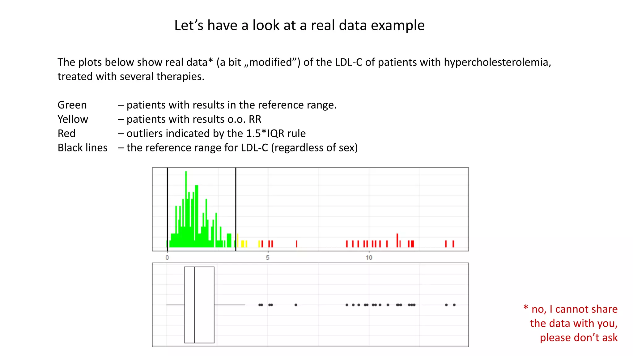
• Severe patient – a patient with a certain clinical parameter exceeding the reference range (e.g. patients with hypercholesterolemia)
• Fake data - data, that are made up during entering it into a database („I don’t have this value… let’s be creative and put 4.23”)
• Data entry error – typos, data copy/pasted from a wrong field, decimal point shifted, too many/few digits, etc.

6. LDL-C HDL-C TG TC TC Friedewald |Δ| (%Δ wrt TCFr) Opinion
110.5 43 120 179 177.5 1.5 (0.8%) OK
120.3 52 130 168 198.3 30.3 (15.3%) query it, just in case
92 32 139 125 151.8 TC < LDL + HDL + TG/5 query it
It was hard to catch, as the
value is in the reference range
and looks good itself.
But, analysed in the context, it
looks suspiciously and should
be confirmed via medical query.
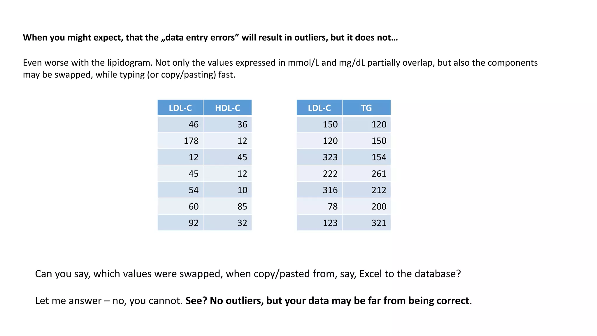
When you might expect, that the „data entry errors” will result in outliers, but it does not…
You might expect, that data entry errors will result in outliers. Say, one put 100.2 rather than 10.02. Or 555 when it should be 5.55.
But what, if the data entry error results in data, that looks perfectly OK?
Let’s have a look at an example of data, that looks correct, but it is not. Let’s consider a lipidogram, consisting of the following parameters:
• Total cholesterol [TC]
• Triglycerides [TG]
• Low-Density Lipoprotein cholesterol [LDL-C]
• High-Density Lipoprotein cholesterol (HDL-C]
Assume, that the patients’ condition allows us to validate the results using the Friedewald formula (results expressed in mg/dL):
TC = LDL-C + HDL-C + TG/5
Now look at the data set below. The values don’t have to match exactly, but should more or less agree

7. When you might expect, that the „data entry errors” will result in outliers, but it does not…
Let’s have a look at another example of data, that may look correct while being not, due to confused units.
Let’s consider the data of patients with anaemia. We will look at the concentration of haemoglobin.
It can be expressed in mmol/L or g/dL. We will look at both.
The reference range is roughly (don’t mind the sex in this example): 12.3 g/dL to 17.5 g/dL (from 7.62 mmol/L to 10.8 mmol/L,
respectively). Patients with serious anaemia start from ca 2 g/dL.
The conversion factor is 0.6206 and makes the reference ranges expressed in both units overlapping.
The problem is, that the values in both ranges agree in meaning (=„serious condition”) only for the smallest values.
Above 7, patients measured in mmol/L are healthy, while patients measured in g/dL are still under severe anaemia. On the picture
below 11 is yellow in both units, but for the opposite reasons (too low in g/dL and to high in mmol/L.
On the next slide you will see what does it mean in practice, if you confuse the units.
g/dL 2 3 4 5 6 7 8 9 10 11 12 13 14 15 16 17
mmol/L 1 2 3 4 5 6 7 8 9 10 11

8. When you might expect, that the „data entry errors” will result in outliers, but it does not…
Here you have a small example of the data with confused units. Let’s assume the unit is provided, but you don’t trust it:
Value Notes
2.48
Regardless of the unit, it indicates severe condition, so it’s hard to decide whether it’s mmol/L
or g/dL at first glance
4.21 Regardless of the unit, it indicates serious anaemia, so it’s hard to detect mismatch
7.11
If these are patients with serious anaemia, it’s rather in g/dL. If your data set contains both
severe and recovering patients, it’s difficult to guess, because 7.11 mmol/L = 11.46g/dL and
this value matches those healthier ones.
8.07
g/dL matches anaemia, while mmol/L means the patient is healthy (=13 g/dL). In anaemia
dataset I’d opt for g/dL
6.17 Now it’s your turn to guess …
8.22 In anaemia trial it’s likely in g/dL
3.65 …
16.21 How did you get this value in anaemia trial?

9. When you might expect, that the „data entry errors” will result in outliers, but it does not…
Even worse with the lipidogram. Not only the values expressed in mmol/L and mg/dL partially overlap, but also the components
may be swapped, while typing (or copy/pasting) fast.
LDL-C HDL-C
46 36
178 12
12 45
45 12
54 10
60 85
92 32
LDL-C TG
150 120
120 150
323 154
222 261
316 212
78 200
123 321
Can you say, which values were swapped, when copy/pasted from, say, Excel to the database?
Let me answer – no, you cannot. See? No outliers, but your data may be far from being correct.

10. Made this quick and dirty, rudimentary illustration long time ago… But I still like it 
Notice: statistical outliers may be totally valid data. And well-looking data may be problematic.

11. Without the context, statistical outlier detection methods would see this
* don’t mind the true distances, number of dots and the distribution, just assume the method(s) correctly detected all outliers. It’s just illustration, not a math formula
Oh, outliers!
Example #1
Example #2
Example #3

12. Those, who propose just „deletion of detected outliers”, propose castration of data
* On the next slides you will see how bad decision it was…
Example #1
Example #2
Example #3
These data are
c a s t r a t e d

13. Technically both are outliers, but clinically OK.
Status: it’s a problem due to unmet inclusion
criteria - both observations are < A
Technically both are outliers.
Clinically o.o RR, but non-significant.
Status: it’s OK
Technically an outlier.
Clinically o.o. RR and significant.
Status: It’s OK
A [inclusion criteria: X must be > A]
Technically an outlier, clinically OK
Status: it’s OK
Technically all are outliers, clinically OK
Status: it’s OK
* Green bands depict reference ranges [RR] covering the normal values in healthy patients
Let’s add some context and observe the status
Context #1 – some fake story about the data (you don’t know). Just look at the statuses to see, how the context changed the meaning of outliers. Tests won’t tell you that.
Context #2
Example #1

14. * Green bands depict reference ranges [RR] covering the normal values in healthy patients
Let’s add some context and observe the status
Context #1
Context #2
Example #2
Technically both are outliers.
Clinically o.o. RR and significant.
Status: it’s OK
Technically OK.
Clinically o.o. RR but non-significant.
Status: it’s OK
Technically OK.
Status: it’s a problem - typo
Technically OK
Status: it’s a problem – confused units
Technically both are outliers.
Clinically o.o. RR and significant.
Status: it’s a problem – typo
Technically all are OK.
Clinically o.o. RR and significant.
Status: it’s a problem due to met
exclusion criteria – X < A
Technically both reds are OK.
Clinically o.o. RR but non- significant.
Status: it’s a problem – confused units or made up data
[exclusion criteria: X < A] A
Technically all those yellow-greens are OK.
Clinically o.o. RR but non-important.
Status: it’s OK

15. * Green bands depict reference ranges [RR] covering the normal values in healthy patients
Let’s add some context and observe the status
Context #1
Context #2
Example #3
In this area all points are clinically o.o. RR and significant.
The circled two are technical outliers, reported by the tests.
Status: it’s OK – only severe patients are recruited in this trial
Technically both are outliers, but clinically OK.
Status: it’s a problem, due to unmet inclusion
criteria: only severe patients are recruited in this trial
Technically outlier, clinically o.o. RR and
important.
Status: it’s a problem - typo
Those are technically OK.
Clinically OK. A few are o.o. RR but non-significant.
Status: it’s a problem – unment inclusion criteria
A [inclusion criteria: X must be > A]
Technically OK, clinically OK
Status: it’s a problem – confused units
Technically an outlier. Clinically OK.
Status: it’s OK
Technically an outlier, but clinically OK.
Status: it’s a problem - typo
Technically outlier, clinically OK
Status: it’s a problem – made up

16. Let’s have a look at a real data example
The plots below show real data* (a bit „modified”) of the LDL-C of patients with hypercholesterolemia,
treated with several therapies.
Green – patients with results in the reference range.
Yellow – patients with results o.o. RR
Red – outliers indicated by the 1.5*IQR rule
Black lines – the reference range for LDL-C (regardless of sex)
* no, I cannot share
the data with you,
please don’t ask

17. 1.5 * IQR 3 * IQR 3 * MAD 3 * SD
skewness - adjusted
1.5 * IQR
Mahalanobis
(z score)
kNN
(Euclidean)
Rosner’s
(ESD)
4.60 - 4.60 - - 0.02 - - -
4.70 - 4.70 - - 0.12 - - -
5.10 - 5.10 - - 0.22 - 5.10 -
5.20 - 5.20 - - 0.23 - 5.20 -
6.39 - 6.39 - - 0.30 - 6.39 -
8.91 8.91 8.91 - - 0.30 8.91 8.91 -
9.22 9.22 9.22 - - 0.36 9.22 - -
9.50 9.50 9.50 - - 0.39 9.50 - -
9.80 9.80 9.80 - 9.80 0.40 9.80 - -
9.90 9.90 9.90 - 9.90 0.40 9.90 - -
10.20 10.20 10.20 - 10.20 0.40 10.20 - -
10.33 10.33 10.33 - 10.33 0.40 10.33 - -
10.54 10.54 10.54 - 10.54 0.40 10.54 - 10.54
10.93 10.93 10.93 - 10.93 0.41 10.93 - 10.93
11.40 11.40 11.40 - 11.40 - 11.40 - 11.40
11.45 11.45 11.45 11.45 11.45 - 11.45 - 11.45
11.56 11.56 11.56 11.56 11.56 - 11.56 - 11.56
11.98 11.98 11.98 11.98 11.98 - 11.98 - 11.98
12.11 12.11 12.11 12.11 12.11 - 12.11 - 12.11
12.23 12.23 12.23 12.23 12.23 - 12.23 - 12.23
13.82 13.82 13.82 13.82 13.82 - 13.82 13.82 13.82
14.20 14.20 14.20 14.20 14.20 - 14.20 14.20 14.20
Outliers detected by various statistical methods
Notes:
1. All the data are correct. No
„problematic” observations
exist in this data set, no
matter what the presented
methods indicate.
2. NOTE 1: The red marked
methods are used „illegally”,
only for illustration purposes.
They all assume that the data
without outliers follow the
normal distribution, which
does NOT hold in our case.
3. NOTE 2: Notice the output of
the skewness-adjusted (via
medcouple estimator)
1.5*IQR (box-plot) method.
It recognized also the
smallest values.

18. Legend
Green: observations in
the reference
range
Yellow: observations out
of the reference
range
Red: outliers
Outliers detected by various statistical methods

19. There were 4 incorrect observations in total:
• 3 green: 1 x copy/pasted from HDL-C, 2 x confused unit
• 1 red: confused unit
Neither of the „outliers” was incorrect just because it’s high (as you might suspect).
How do you think, where were the problematic observations?

20. One might say, that the outlier detection methods certainly helped us to differentiate the patients with good
response to the therapies (= who have lowered their LDL-C) from those, who do not.
Well, yes - to some extent. Recall what I said about possible reasons of the skewness – it may indicate mixed
observations from 2+ populations, not separated by any covariate.
But it wasn’t so clear in this case. Some patients didn’t respond to the therapy well (for various reasons),
while, at the same time, some patients with high initial LDL-C (520 mg/dL; homozygous familial
hypercholesterolemia) were able to reduce their LDL-C, still having it high (380 mg/dL).
See? Without the context, your guesses may (WILL) deceive you.
Don’t the outlier detection procedures do something useful for us?

21. How do you think, where were the problematic observations?
Good response,
despite high LDL-C
Something went
wrong…

22. What you should learn
1. I told you a lot of stories about the presented data. I gave you the context. Without the context, some
might just see just a „garbage to clean”. You saw there was no garbage in the data.
2. With the context attached, it turned out, that the issues were not in the place you might expect them.
3. In real life, especially in data science, you may not know the history of the analysed data, thus, you may
not know the context.
4. Even then – don’t rely on the outlier detection methods blindly and don’t follow „gurus” telling you to
„remove the garbage” thoughtlessly. The only garbage here are their advises.
5. Always make the effort and try to learn something about the data: its origin, its nature. Search the
literature and the Internet for confirmation. Don’t „assume”, don’t „guess” . Ask the domain experts.

23. If you have to deal with outliers
1. Sometimes you will have to exclude outliers (errors, single justified cases). Never do that automatically. If
you cannot justify the exclusion convincingly, just – don’t.
2. If you have more outliers, try to:
a) Explain their origin and nature. They may be (often are) perfectly valid data
b) Revise your model. Think od adding a covariate, which will separate your data into sub-groups. You
may find, that the data in both groups is much more homogenic, but differ in dispersion (variance).
See the illustration with an example of such situation on the next slide.
• I also like the idea of employing classification trees to detect outliers. If the outliers fall into a
separate leaf (leaves), you won and get the „decision rule” on how to get there.

24. If you have to deal with outliers

25. 2. If you have more outliers, try to:
…
c) Embrace appropriate statistical methods. Come on, it’s XXI century. Use the Force (Internet), Luke.
E.g. Namboodiri KK, Elston RC, Glueck CJ, Fallat R, Buncher CR, Tsang R. Bivariate analyses of cholesterol and triglyceride levels in
families in which probands have type IIb lipoprotein phenotype. Am J Hum Genet. 1975;27(4):454‐471.
https://www.ncbi.nlm.nih.gov/pmc/articles/PMC1762792/
d) Your data seem clean now? Don’t let it fool you! Validate the „correct” data too, if only possible.
Remember overlapping reference ranges? Swapped values?
e) Remember, that outliers may be multi-dimensional. As such, you may not be able to see them using
single-dimensional tools.
If you have to deal with outliers

26. I know some of you will ask me for the R packages I used. Here you are:
1. https://cran.r-project.org/web/packages/outliers/
2. https://cran.r-project.org/web/packages/OutlierDetection
3. https://cran.r-project.org/web/packages/EnvStats (Rosner’s test)
4. https://cran.r-project.org/web/packages/robustbase/
Hubert, M. and Vandervieren, E. (2008). An adjusted boxplot for skewed distributions,Computational Statistics and Data
Analysis52, 5186–5201, https://wis.kuleuven.be/stat/robust/papers/2008/adjboxplot-revision.pdf